


Joanne Blanden
University College London
Submitted for PhD in Economics,
Final Version, October 2005
Abstract
This thesis focuses on how the economic status of children is related to their parental income.
I begin by measuring the intergenerational earnings mobility of sons in a comparative framework. I compare the extent of earnings mobility for sons in the UK, US, West Germany and Canada, and consider how mobility has changed across time in the UK and US. I find that while it is difficult to statistically distinguish between estimates, it appears that the UK and US are less mobile than the other countries. When looking over time, there is definitive evidence that mobility for sons in the UK has declined, while there is no such evidence for the US.
There is a clear connection between the persistence of income inequality across generations and the unequal distribution of educational attainments. I show that part of the decline in mobility in the UK is due to increasingly unequal access to higher education.
The majority of the literature on intergenerational mobility stresses the relationship between individual earnings and parental income. But economic wellbeing also depends on the earnings and income of partners. If partner’s income is strongly connected with parental income this will reinforce individual earnings persistence. Assortative mating is the extent to which people with similar characteristics form couples, and this has a crucial role here in explaining the link between partners and parents.
The final section of this thesis explores the role of assortative mating in intergenerational mobility. For the UK, I demonstrate that the increasing association between parental incomes and the earnings of daughters-in-law substantially adds to the relationship between sons’ and their parents’ family incomes. For Canada, I am able to link the incomes of both sets of parents for the couple. I demonstrate that the association between parental incomes within the couple is a new measure of assortative mating and show that couples who are less similar in terms of their parental income are more likely to separate.
Contents
Acknowledgments
Chapter 1: Introduction
Chapter 2: Literature Survey: The Theory and Measurement of Intergenerational Persistence
2.1 Introduction
2.2 The Theory of Individual Income Persistence
2.3 Measurement Methodology
2.4 Summary of Current Findings on Intergenerational Mobility for Sons
2.5 Theoretical Background on Assortative Mating and Family Income Persistence
2.6 Measuring the Contribution of Assortative Mating to Intergenerational Persistence
2.7 Results from the Intergenerational Mobility and Assortative Mating Literature
2.8 Conclusion
Chapter 3: International Evidence on Intergenerational Mobility
3.1 Introduction
3.2 Empirical Approach
3.3 Data
3.4 Comparative Measures of Intergenerational Mobility
3.5 Decomposing Intergenerational Mobility
3.6 Conclusion
Appendix to Chapter
A.3.1.Qualifications Categories
Chapter 4: Changes in Intergenerational Mobility in the UK and US
4.1 Introduction
4.2 Current Evidence
4.3 Data
4.4 Estimation Approaches
4.5 Changes in Intergenerational Mobility in the UK
4.6 Changes in Intergenerational Mobility in the US
4.7 Discussion
4.8 Conclusion
Chapter 5: The Role of Education in Generating Increased Intergenerational Persistence in the UK
5.1 Introduction
5.2 Education Policy in the UK
5.3 Data
5.4 Changes in Intergenerational Mobility and Educational Inequality
5.5 Robustness Checks on Educational Inequality
5.6 Methods to Establish Causality in the Relationship between Parental Income and Education
5.7 The Causal Impact of Parental Income on Education
5.8 Conclusion
Chapter 6: Intergenerational Mobility and Assortative Mating in the UK
6.1 Introduction
6.2 Theoretical Background and Measurement Issues
6.3 Data 6.4 Changes in Assortative Mating
6.5 Education and Parental Income
6.6 Results on Changes in Intergenerational Mobility
6.7 Discussion
6.8 Conclusion
Appendix to Chapter
A.6.1 First-stage Regressions for Heckman Corrections Accounting for Selection
Chapter 7: Assortative Mating on Parental Income – Love and Money
7.1 Introduction
7.2 Theoretical Background and Estimation Issues
7.3 Data and Description of Matching Procedure
7.4 Results on Intergenerational Mobility
7.5 Results on Assortative Mating
7.6 Conclusion
Appendix to Chapter 7
A.7.1. Additional Descriptive Statistics
Chapter 8: Conclusions
Appendix: Attrition and Item Non-response in the British Cohort Studies
A. 1 Introduction
A.2 The Problem of Attrition and Non-response
A.3 Evidence on Sample Attrition in Other Datasets Used
A.4 Description of Attrition and Non-response in the Cohort Studies
A.5 Conclusions
References
List of Tables
2.1 Summary of Literature on Intergenerational Persistence for Sons, US
2.2 Summary of International Literature on Intergenerational Persistence for Sons
2.3 Summary of Literature on Changes on Intergenerational Persistence
2.4 Summary of Literature on Intergenerational Persistence in Daughters’ Earnings, Family Income and Partners’ Earnings
3.1 Summary of Comparative Samples
3.2 Descriptive Statistics for Comparative Samples
3.3 Comparisons of Intergenerational Mobility Based on Parental Income
3.4 Comparisons of Intergenerational Mobility Based on Fathers’ Eamings
3.5 Transition Matrix for the UK
3.6 Transition Matrix for the US
3.7 Transition Matrix for West Germany
3.8 Transition Matrix for Canada
3.9 Descriptive Statistics for Education
3.10 Returns to Education
3.11 Educational Decompositions
A.3.1 Qualifications Categories
4.1 Descriptive Statistics for UK Samples
4.2 Changes in Intergenerational Mobility in the UK
4.3 Measurement Error Calibrations for the UK
4.4 Descriptive Statistics for the Three Cohort Approach to the PSID
4.5 Three Cohort Approach to Measuring Changing Mobility in the US
4.6 Sample Sizes for Mayer-Lopoo Replication
4.7 Variations on Replicating the Mayer-Lopoo Approach to Changing Mobility in the US
4.8 Changes in Earnings Mobility in the US: Replication and New Results
5.1 Descriptive Statistics on Education and Parental Income
5.2 Education and the Intergenerational Mobility of Sons 5.3 Staying on at School and Parental Income, Cohort Data
5.4 Staying on at School and Parental Income, FES Data
5.5 Degree Acquisition by Age 23 and Parental Income
5.6 Using Consumption Data to Test Staying on and Parental Income Relationships
5.7 Testing Alternative Income Specifications
5.8 Adding Controls to Models of Educational Inequality
5.9 Relationships between Educational Attainment and Income at 16: Controlling for Sibling Fixed Effects using the BHPS
5.10 Relationships between Educational Attainment and Income at 16: Controlling for Permanent Income using the BHPS
6.1 Characteristics of Samples by Partnership Status
6.2A Assortative Matching on Age Left Full Time Education, Sons
6.2B Assortative Matching on Age Left Full Time Education, Daughters
6.3 Relationships between Education and Parental Income
6.4 Estimates of Earnings Mobility by Gender and Partnership Status
6.5 Household Composition and Earnings Shares
6.6 Household Earnings Mobility for those with Partners
6.7 Intergenerational Parameters for Full-Time Employed Women Only
6.8 Parental Income and Participation
6.9 The Earnings Mobility of Women – Correcting for Endogenous Participation
6.10 Estimates of Earnings Mobility for Cohort Members and Their Households, Married Sample
A.6.1 First-stage Regressions for Heckman Corrections Accounting For the Selection into Employment
A.6.2 First-stage Regressions for Heckman Corrections Accounting For the Selection into Full-Time Employment
7.1 Number of Daughters Matched 227
7.2 Characteristics of the Matched Sample Compared With All Women in the HD
7.3 Characteristics of Women in the SLID in 1998
7.4 Intergenerational Mobility in Canada by Gender and Partnership Status
7.5 Intergenerational Mobility and Assortative Mating
7.6 The Education Levels of Couples in the SLID
7.7 Evidence for Assortative Mating on Education from the SLID
7.8 Measures of Assortative Mating on Earnings and Income
7.9 Variations in Assortative Mating by Characteristics
7.10 Descriptive Statistics for Divorce and Separation
7.11 Assortative Mating, Divorce and Separation, Post-1992 Partnerships
7.12 Assortative Mating and Divorce for Those Ever Married
A.7.1 Descriptive Statistics for the Couples Sample
A.7.2 Divorce Rates by Parents’ Income Quintiles
A.7.3 Threshold Effects and Divorce
A.l Attrition in the Cohort Studies
A.2 Item Non-response in the Cohort Studies
A.3 The Combined Effect of Attrition and Non-Response
A.4 The Impact of Attrition and Non-Response on Sample Characteristics – NCDS
A.5A The Impact of Attrition and Non-Response on Sample Characteristics – BCS Males
A.5B The Impact of Attrition and Non-Response on Sample Characteristics – BCS Females
List of Figures
3.1 Male Earnings Profile in the UK
3.2 Male Earnings Profile in the US
3.3 Male Earnings Profile in West Germany
3.4 Male Earnings Profile in Canada
4.1 Mayer and Lopoo Results Compared with my Replication
4.2 Earnings and Family Income Mobility Compared using MayerLopoo Approach
4.3 Intergenerational Earnings Coefficients: Replication and New Results
4.4 Intergenerational Earnings Correlations: Replication and New Results
5.1 Changes in Educational Attainment and Participation in the UK
5.2 Student Maintenance Grants in 1976/1977
5.3 Student Maintenance Grants in 1988/1989
5.4 Student Maintenance Grants and Loans 1980/1981 to 2001/2002
6.1 Age Formed Current Partnership, Males
6.2 Age Formed Current Partnership, Females
Statement of Conjoint Work
% Contributed by Candidate
Chapter 1: Introduction 100%
Chapter 2: Literature Survey: The Theory and Measurement of Intergenerational Persistence 100%
Chapter 3: International Evidence on Intergenerational Mobility 100%
Chapter 4: Changes in Intergenerational Mobility in the UK and US 50%
Chapter 5: The Role of Education in Generating Increased Intergenerational Persistence in the UK 33%
Chapter 6: Intergenerational Mobility and Assortative Mating in the UK 100%
Chapter 7: Assortative Mating on Parental Income – Love and Money 100%
Chapter 8: Conclusions 100%
I certify that this is an accurate statement of the candidate’s contribution to the research described in this thesis.
Supervisor’s signature…. ………………………………………….. Date.28/10/05
Acknowledgements
First, I would like to thank my supervisor Stephen Machin. He encouraged me to continue my studies after my MSc and has been an invaluable mentor throughout the PhD. Steve provided the impetus behind this research agenda, worked with me on the early papers and allowed me the time to bring this thesis to fruition. I really appreciate it. Paul Gregg has also been an important mentor and collaborator, from whom I have learned a lot. I have also benefited from the comments and teaching of the faculty at UCL, especially Costas Meghir and Christian Dustmann.
The Centre for Economic Performance has been an incredibly supportive employer throughout my studies, and I would like to thank the CEP manager Nigel Rogers and the director, John Van Reenen. I especially appreciate the opportunity to travel to Canada to work on the data used in Chapter 7.
My visits to Canada were made as part of Statistics Canada’s PhD stipend programme and I am therefore grateful to Statistics Canada and to Miles Corak for arranging this. I am also grateful to Miles and to Sophie Lefebvre for their help in using the IID data. Delia Carley must also be thanked for looking after me so well in Ottawa.
The British data used in this thesis was made available by the Data Archive. I am appreciative of the work of those at the Centre for Longitudinal Studies who oversee the British cohort studies, of which I make extensive use. Alissa Goodman at the Institute for Fiscal Studies answered many appeals for help with the cohort data. I am grateful to DIW in Berlin for granting access to the German Socio-Economic Panel. Tanvi Desai at the CEP played a crucial role in providing easy access to and use of the data.
I am extremely grateful to the members of the CEP for being such generous colleagues. Numerous individuals have provided help and advice (sometimes far beyond the call of duty), especially Sandra McNally, Guilia Faggio, Teresa Casey, Chris Crowe, Olivier Marie, Richard Belfield, Becky Givan, Joan Wilson, Shqiponja Telhaj, Steve Gibbons, Jonathon Wadsworth, Richard Dickens and Steve McIntosh. As well as providing support, many of my colleagues at CEP have also become great friends, and I hope they will continue to be so. My friends on the outside, Jasmine Fletcher and Lucy White also deserve thanks, as does my landlord, Anthony Mortimer, both for his generosity and for providing amusement after a long day at the office.
My parents, Joan and Barry, have been very encouraging throughout my studies. Needless to say, it would not have been possible without them. Last of all, I would like to thank Steve Morey who has borne the brunt of my trials and tribulations over the past two years. Billy Bragg once said ‘Scholarship is the Enemy of Romance’. I’m glad that hasn’t been true.
Chapter 1: Introduction
Intergenerational mobility is concerned with the relationship between the socioeconomic status of parents (often their income) and the economic outcomes of their children as adults. Most commonly, this is measured as the association of incomes across generations. A strong association between incomes across generations indicates weak intergenerational income mobility, and is often regarded as in violation of the norms of equality of opportunity. If an individual’s income is strongly related to his or her parents’ income, this means that a child from a poor family has limited opportunities to escape his or her start in life; consequently inequality perpetuates. This has implications for economic efficiency if the talents of those from poorer families are under-developed or not fully utilised, as those from poorer backgrounds will not live up to their productive potential.
The connection between intergenerational mobility and equality of opportunity means that the extent of the association between the incomes of parents and children is a topic of strong policy interest. Indeed, a recent piece in the Economist has pointed to the identification of high intergenerational mobility with the concept of the ‘American Dream’,
Americans believed that equality of opportunity gave them an edge
over the Old World, freeing them from debilitating snobberies and at
the same time enabling everyone to benefit from the abilities of the
entire population. They still do1.
Most people would agree that equality of opportunity is an important goal; nonetheless, it is difficult to imagine a world with no link between incomes across generations. Genetic transmissions alone are likely to lead to a positive association between the earning power of parents and children2 and the transmission of family culture and other learning within the family will lead to children from better off families being better equipped to succeed. These effects may be more important than the direct influence of income, through richer parents being able to make more investments in goods and services for their children.
1 Economist December 29th 2004.
2 For example, Perisco, Postlewaite and Silverman (2004) describe the positive earnings premium to being tall and of having tall parents.
As Corak (2004) points out, this means that the policy implications of the study of intergenerational mobility are unclear. If intergenerational income inequality is solely a consequence of the automatic transmissions of ability and other attributes within the family, the reduction of these inequalities would require strong intervention by the state. Our understanding of this can be improved by making comparisons of the levels of intergenerational mobility across time, place and groups. With comparisons in hand, it is possible to assess mobility as ‘relatively weak’ and ‘relatively strong’, and therefore begin to consider potential explanations for differences in intergenerational mobility.
Making comparisons of mobility is at the heart of much of the empirical work in this thesis; in order to do this convincingly, careful attention to methodology is paramount. One of the themes which runs through my research is how the available data can be best used to avoid the biases inherent in measuring intergenerational persistence, or at least how careful estimation can be used to ensure that biases are similar across the groups under comparison.
The majority of my analysis is focused on the measurement of the intergenerational elasticity, p and the intergenerational correlation, r. These parameters are obtained from the estimation of a double-log regression (see equation (1.1)) of the earnings of sons (or in the later chapters daughters and children’s partners), ln^.”” on the income of their parents, \nYiparerus. Larger p and r indicate less intergenerational mobility. Issues concerning the theoretical motivation behind this model and its measurement will be considered in detail in Chapter 2.![]()

Differences in the variance of InK between generations will distort P which is why the intergenerational partial correlation is also considered throughout. This is obtained simply by scaling p by the ratio of the standard deviation of parents’ income to the standard deviation of sons’ income, as shown in equation 1.2.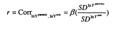

The first two chapters of my empirical analysis (Chapters 3 and 4) are concerned with measuring the intergenerational earnings mobility of sons in a comparative framework. There are two motivations here; the first is simply to describe how intergenerational mobility varies over time and place. For example, do levels of intergenerational mobility in the US, compared with Europe, match up with the story of the ‘American Dream’ described above? The second motivation is more analytical, by comparing intergenerational mobility across countries and over time, it is hoped that more can be understood about how intergenerational mobility varies across different institutional and policy environments.
More formally, comparisons of r over countries and time are equivalent to estimating r. and rk where j and k indicate different time periods or countries. Making comparisons is equivalent to estimating {rk – r – ) , the exercise then is to consider the differences in other characteristics which could explain the differences found in mobility. In Chapter 5, I consider the role of education in explaining changes over time in mobility (between rt and rl+l) for the UK.
Chapter 3 studies intergenerational mobility for sons in the US, the UK, West Germany and Canada, where sons’ earnings are measured around 2000, when they are aged approximately 30. A previous limitation of cross-country comparisons has been the difficulty of comparing results from different studies, as methodological factors may be responsible for the differences found between studies. My aim in this chapter is to fill this lacuna and demonstrate the extent to which the conclusions from a comparative study differ from those which can be drawn from the current literature.
There is a clear connection between the persistence of income inequality across generations and the unequal distribution of educational attainments. Young people from well-off families get more education than their poorer peers, and this is one of the reasons for their higher earnings. The extent to which education is responsible for intergenerational persistence depends on how strongly educational attainment is tied to family income background and on the rewards to education in the labour market. In Chapter 3 ,1 expand the descriptive aspect of my analysis by decomposing the levels of intergenerational persistence for the UK, US and West Germany. This involves comparing the extent to which persistence is associated with differences in education levels.
Chapter 4 considers changes in mobility over time for the UK and US. In the UK this analysis relies on comparing two sources of data, the 1958 and 1970 British birth cohorts. The analysis for the US relies on the Panel Study of Income Dynamics. The advantage of the US data is that information is available for all cohorts of individuals bom between 1949 and 1970; however the limitation is that the effective sample sizes are small compared with those available for the UK.
The objectives in this chapter are similar to those for the cross country comparisons of levels of mobility, and once again measurement issues are paramount. While the changes in intergenerational mobility in the two countries are interesting in themselves, there is a clear expectation that by comparing trends across two countries it is possible to learn more about how policy or institutional changes underpin the trends. A particular aspect of interest is the strong growth in cross sectional inequality experienced in the two countries over the time period under consideration. The literature has tended to posit an informal link between cross-sectional income inequality and intergenerational income persistence (Hout 2004); it is therefore particularly interesting to discover if increasing inequality is associated with falls in mobility.
In Chapter 5 I return to the role of educational attainment and study its contribution to intergenerational mobility and its change over time in the UK. Considering the role of educational attainment is highly relevant in a policy context. Education is assumed by many to be ‘a great leveller’. Consequently, attempts to improve the education of children from poor backgrounds are one of the main ways that Governments intervene to weaken intergenerational persistence. Chapter 5 therefore makes the most policy oriented contribution.
My analysis in Chapter 5 is two-fold. The objective of the first part of the chapter is to model the changing relationship between family income and educational attainment between the 1970s and the present. This enables me to assess both how the connection between family income and education are linked with changes in intergenerational mobility in the UK, and to develop an insight into patterns of intergenerational transmission among more recent cohorts. I find that differences in education by parental income are an important reason for intergenerational persistence. In the second part of my analysis, I attempt to understand what leads to gaps in educational attainment by family income. My objective is to separate the effects of ability and family culture from the direct effect of income.
As discussed in the opening paragraph, the concepts of intergenerational mobility and persistence are concerned with the correlation between economic status across generations. The first three empirical chapters of the thesis are concerned with individual-level intergenerational mobility, with the outcome measure being the earnings or education level of young adults. But economic well-being is a broader concept than individual earnings and is likely to depend on the earnings and income of partners as well as the individual’s own income. The second section of my thesis (Chapters 6 and 7) adds an analysis of household formation to my investigation of intergenerational mobility.
If partners’ incomes are as strongly correlated with parental income as the individuals’ own earnings are, this will reinforce individual earnings persistence and mean that family income persistence is even stronger. This is the premise behind the consideration of the role of household formation in intergenerational mobility explored in Chapter 6 for the UK, and Chapter 7 for Canada. The relationship between partners’ earnings and parental income is mediated through assortative mating; the extent to which couples match on the basis of having similar characteristics, and I explore this explicitly in both chapters.
In Chapter 6 I model family income mobility in Britain for the 1958 and 1970 cohorts. I consider the role of partnership formation in adding to intergenerational family income inequalities, and illustrate the role played by wives and partners in contributing to trends in intergenerational mobility. Previous studies of this topic have focused on the importance of husbands in contributing to the persistence of income for women; in this chapter I perform a symmetric analysis for both men and women. This draws attention to the role of partners in contributing to the intergenerational persistence of men; an aspect which has not previously been stressed.
It is clear that household formation and assortative mating has an important role in generating the strong persistence in family income in the UK. In the final empirical chapter of this thesis I am able to compare the findings obtained in the UK with a similar analysis for Canada. This reintroduces the comparative aspect of the earlier chapters.
The unique data used to capture intergenerational relationships in Canada enables a new dimension in assortative mating to be explored. The Canadian Intergenerational Income Data is based on linked tax returns and includes information on the incomes and earnings of couples, as well as the incomes of both sets of parents during the couples’ teenage years. A new measure of assortative mating is proposed; the link between the incomes of parents-in-law. This shows that the interrelation between household formation and intergenerational mobility is two-sided. Not only does household formation affect intergenerational mobility through partners’ earnings, but parental characteristics also influence how couples match.
The final dimension of my interrogation of the Canadian data is to explore how matching on parental incomes varies according to different characteristics. I test insights from search models of household formation, specifically the hypothesis that individuals with higher search costs match more weakly on parental income. I also assess if couples who are well matched on parental income are less likely to separate.
This thesis therefore provides a thorough consideration of a number of interlinked aspects of intergenerational mobility, in the UK and in other countries. I emphasise a comparative approach throughout, and discuss how intergenerational mobility varies across countries, time, and gender. In addition, several of my chapters discuss how education acts as a transmission mechanism between the incomes of parents and children; this enables me to focus more sharply on the policy implications of my findings.
In the next chapter I precede the empirical chapters with a review of the literature. This develops the economic approach to explaining intergenerational persistence and demonstrates the ways that the measurement of mobility has developed in order to minimise the biases inherent in its estimation.
Chapter 2: Literature Survey: The Theory and Measurement of Intergenerational Persistence
2.1 Introduction
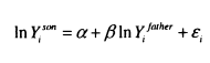
Much of the empirical work included in this thesis focuses around the estimation of P in the following regression;
![]()

where In Ytch,ldren is the log of some measure of earnings or income for adult children, and In Ylparen,s is the log of income for parents, i identifies the family to which parents and children belong and et is an error term, ft is therefore the elasticity of children’s income with respect to their parents’ income and ( l- fi) can be thought of as measuring intergenerational mobility3.
Hypothetically, P = 0 represents a case of complete mobility where the incomes of parents and children are completely unrelated and ft – 1 represents a case of complete immobility where the proportionate earnings advantage of parents is precisely mirrored in their children’s generation. If p > \ the income advantage of parents is magnified in the child’s generation, meaning that over generations the incomes of dynasties become increasingly unequal. In general, empirical estimates of p tend to lie between 0 and 1, implying that an initial income advantage will be wiped out over several generations – regression to the mean.
In this chapter, I provide a survey of the literature to set the scene for the empirical chapters that follow. I discuss the theoretical motivation behind the estimation of equation (2.1) in the case where In is the child’s individual earnings and for the broader case considered in Chapters 6 and 7, where In Yich,ldren is the child’s partner’s earnings or his/her family income. I also highlight the role that human capital plays in the theoretical models of income persistence across generations; this motivates the investigation of the role of education as a transmission mechanism which occurs in Chapters 3 and 5.
3 The regression approach to measuring connections across generations dates back to Galton’s (1886) consideration of height.
This thesis is to a large extent based on empirical studies of intergenerational mobility, it is therefore very important to fully understand the difficulties and biases inherent in measuring intergenerational persistence. As the empirical side of the literature has developed, researchers have continued to improve the methodology used and to consequently obtain better estimates of mobility. I therefore review what the literature has taught us so far about measuring intergenerational mobility, and obtaining an unbiased and consistent estimate of in equation (2.1)
I also summarise a selection of the results from the empirical work carried out thus far. I focus on the studies with the most convincing methodologies, and those with the most relevance to my own work. I show how the estimates of intergenerational mobility in the US have evolved as measurement methods have improved, before demonstrating the extent to which the current literature indicates variation in intergenerational mobility over countries and across time. I also review the current literature on persistence between parents and daughters and children’s partners and their parents, which is a much less developed area of study. My approach to this review is to examine the theory, measurement and empirical work for individual mobility first, and then to follow this with a discussion of assortative mating and family income mobility.
2.2 The Theory of Individual Income Persistence
In this section I review how economic theory interprets intergenerational transmissions, and discuss the insights gained by modelling intergenerational transmissions within a utility maximising framework.
The main economic model of intergenerational mobility is formulated in Becker and Tomes (1986). In their model, parents choose the optimal investment to make in their children by maximising their utility function. Equation (2.2) shows that parental utility (Uil_l ) is generated by parents’ own consumption ( CJf_,) and the consumption of children in the next generation ( Cit). The extent to which parents care about their children’s consumption is represented by the parameters; if s = 0 parents care only about their own consumption, while if 71 – 1 they care only about their children’s consumption, ^therefore indicates the extent of parental altruism.
![]()

The income of children is determined by the amount of human capital which parents have invested (/.,), the return on these investments (</>), their endowments ( Elt), the return to endowments (rj) and by an error, uit which represents market luck, as shown in equation (2.3).
![]()

The children’s endowment Eit, will also be influenced by intergenerational factors. A proportion of the endowment is transmitted from parents to children regardless of investment decisions. This is shown in equation (2.4) where h represents the extent of the endowment’s heritability within the family.
![]()

As parental income is a function of parents’ own endowments (through equation 2.5), the inheritance of endowments alone will be sufficient to generate intergenerational persistence in income.
![]()

Parents decide on the level of human capital on the basis of their degree of altruism, the resources they have available, and the return to the investment. In their discussion of the contribution of economic theory to the understanding of intergenerational mobility, Grawe and Mulligan (2002) emphasise the importance of price. It is the sensitivity of parental behaviour to prices (the costs and benefits of human capital investment), which marks out economic models of inheritance from those which are simply due to the transmission of endowments.
The implications of the human capital investment model for the relationship between earnings and consumption across generations depend upon the budget constraint faced by parents. If capital markets are perfect, parents can borrow on their children’s behalf and pass the debt between generations. In this framework investment in human capital will be unaffected by parental income, and the intergenerational transmission of earnings will be equal to the heritability of endowments. Earnings will regress to the mean across generations because endowments are not fully inherited. However, parents will offset this by asset transfers to children; this implies that consumption does not regress to the mean.
In this case, the relationship between the child’s income and their parental income is determined entirely by the heritability of endowments and by the reward to endowments for parents and children – combining equations (2.3), (2.4) and (2.5) gives equation (2.6).
![]()

If the returns to endowments are equal across generations, the intergenerational correlation of income will simply be equal to h , the heritability of endowments. It is also clear that human capital is unrelated to parental income, consequently this T) aspect is included in the error, such that 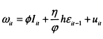

If capital markets are imperfect, so that parents cannot borrow to finance human capital, the model has rather different implications. All investments in human capital must be funded from parental income, and some parents will not be able to make the optimal investment. This adds a new dimension to the intergenerational income relationship, for constrained families, human capital will be a function of parental income. In this case, intergenerational transmissions will be due to both endowment transmissions and human capital investment.
In a model with credit constraints, there will be two groups of families with quite different intergenerational transmissions. The first group will be unconstrained and will therefore behave like families under the intergenerational permanent income model; earnings will regress to the mean while consumption will not. For the second group, who are constrained, earnings will regress more slowly to the mean. The extent of intergenerational persistence for the second group will be strongly dependent on the returns to human capital, expressed as $ in equation (2.3).
Both Goldberger (1989) and Mulligan (1997, 1999) point out that economic models are unhelpful if they cannot be distinguished from a mechanical approach to persistence driven only by endowments. Mulligan (1999) takes several of the predictions of the credit constraint model to the data. In particular he attempts to identify families who are borrowing constrained and discover if they differ from unconstrained families in the ways predicted by Becker and Tomes. His results are mixed.
In an alternative approach, Grawe (2004a) has emphasised the interaction between income and ability in leading to credit constraints. Credit constraints exist when financial limitations mean that families cannot afford optimal investments; this will occur when sons have high ability relative to their parental income. Quantile regressions show up variation in the intergenerational relationship by son’s earnings, conditional on parental income. If a son’s earnings are high compared to parental income, we can assume he is bright. Therefore more intergenerational persistence at higher quantiles is indicative of credit constraints. Grawe finds no evidence of credit constraints in Canada on the basis of this test.
Many empirical models of intergenerational persistence stress the importance of educational attainment, doubtless in part, because of Becker’s emphasis on human capital investment. However, as I have shown in this discussion, noting the importance of education does not have much theoretical weight. This is because the relationship between educational attainment and family income can be due to either differences in inherited endowments or differences in parental investments; it is not straightforward to distinguish between the two explanations. In Chapter 5 I discuss the mediating role of education and attempt to separate the role of income from endowments in generating education differences by parental income.
Solon’s (2004) model builds on the Becker and Tomes approach to highlight the factors which may underlie differences in intergenerational mobility across countries and over time. The crucial development made by Solon is that the role of the state in making investments in children is made explicit. In Solon’s model there is no transfer of debts or bequests, parental income must either be consumed or spent on the human capital of children. This is equivalent to Becker and Tomes (1986) imperfect capital market formulation.
A child’s final human capital depends on his or her endowments, the investments made by parents and the investments made by the state. Parents’ investments are substitutes for government investment; more progressive investment by the government means a weaker connection between final human capital and parental income. The connection between human capital and parental income will be stronger if endowments are strongly heritable across generations, if parents’ investments in human capital are more efficient, and if expected returns to investment are higher.
To sum up, some intergenerational persistence is always anticipated if income-earning endowments have an inherited component. Additional intergenerational persistence will occur if capital markets are imperfect so that parents are unable to make optimal investments in their children’s human capital. In this case, the return to human capital is responsible for the transmission of differences in human capital into differences in sons’ adult incomes. It is therefore clear that stronger returns to human capital will lead to more persistence in incomes across generations. Solon’s model adds the role of government investments to this story. Consequently, when considering differences in intergenerational mobility across time and place, differences in government education policy and differences in the returns to education seem natural starting points; both of these will be considered in the body of the thesis.
2.3 Measurement Methodology
The parameter of interest is the intergenerational elasticity (fi) which is the regression coefficient on father’s economic status in a model of son’s adult economic status (both are generally measured by either earnings or income)4. A higher elasticity indicates that fathers’ incomes are more closely linked to sons’ economic success, meaning higher intergenerational inequality. The intergenerational elasticity is estimated by running a linear regression of sons’ income of parents’ income, as in equation (2.7).
4 In this thesis I am concerned with persistence from parents to sons, daughters, and sons-in-law and daughters-in-law. Many of the same issues are relevant throughout, so here I discuss the relationship between fathers and sons as this has received most attention in the literature.

Given the theoretical discussion provided in the previous section, it is clear that the variables we would like to use in this regression would be fathers’ and sons’ permanent incomes. The difficulties caused by the fact that permanent income is not observed are a recurring theme throughout the intergenerational literature.
The standard model of measurement error which underpins the discussion of this issue in Solon (1992) and Zimmerman (1992), states that current income is related to permanent income as shown in equation (2.8), such that current income ( y’it) deviates from permanent income according to some random error. This measurement error takes the same form for both the child’s and parents’ generations.
![]()

Under classical measurement error assumptions , it is straightforward to show that measurement error in the dependent variable (the child’s income) will not affect the bias of the estimate of /?, although it will lead to a loss of precision and larger standard errors. However, measurement error in the explanatory variable has more serious implications, and will lead to inconsistent estimates of /?. Indeed, the estimated parameter, f t , will be an underestimate of the true /?, as shown in equation (2.9), where crj and cr] are the variances of permanent income and the error respectively.
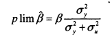

It is clear that the magnitude of the ‘signal to noise’ ratio is crucial to obtaining accurate estimates of intergenerational persistence. If the variance of error contained in y * f is small compared to the true variance then ft will be
5 These assumptions are that yt- and ui{ are uncorrelated, and that measurement error is
uncorrelated across generations
close to /? and we will have a good estimate of intergenerational persistence. Minimising the extent of measurement error is a priority for intergenerational mobility research, and it is an issue that both Solon (1992) and Zimmerman (1992), and indeed many papers which follow them, consider in detail.
The first step taken to overcome this problem is to model current income as a function of permanent income and age, as in equation (2.10). If the age and age-squared of both fathers and sons is added to the regression the age-related difference between current income and permanent income will be conditioned out. I therefore add appropriate age controls to all my models. Nonetheless, this is likely to move the estimates only a small step closer to reflecting permanent income.
![]()

Another contribution made by Solon and Zimmerman is to draw attention to the impact of unrepresentative samples for estimates. Owing to the problems involved in obtaining any information about incomes in two generations, unrepresentative samples were a feature of the early empirical studies of intergenerational mobility. Behrman and Taubman (1985) use a sample of fathers drawn from white male twins who served in the military, while Sewell and Hauser (1975) use a sample of Wisconsin High School Seniors from 1957. The pioneering study of intergenerational mobility in the UK (Atkinson 1981 and Atkinson et al 1983) used a sample of parents living in York in 1951 and excluded higher income families. Solon (1992) points out that measurement error bias will be compounded if the samples of fathers are not representative, as this will lead to a reduced variance of income. In equation (2.9) which demonstrates the impact of measurement error, s2 will be the estimate of a 2 and if s2 < a 2 there will be a lower ratio of signal to noise, exacerbating attenuation bias. The use of nationally representative samples has become standard in more recent mobility studies.
The studies by Solon and Zimmerman seek to alleviate the twin difficulties of homogenous samples and measurement error. Both studies are based on nationally representative samples (the first from the Panel Study of Income Dynamics, the second from the National Longitudinal Surveys), and both seek to minimise measurement error by averaging father’s earnings over four or five years of annual data. Under the classical measurement error model there will be a fall in the attenuating factor as more periods of data are used to generate the average, as shown in equation (2.11). As T approaches infinity, will converge to zero and ft will approach the true value of .

I shall discuss the results from Solon’s and Zimmerman’s papers in detail below. However, what is clear from these papers is that measurement error in father’s earnings can produce estimates of the intergenerational elasticity that are biased downwards; what is less clear is whether a four or five-year average of income is sufficient to overcome this problem. An alternative solution to the classical measurement error problem is to use instrumental variables (IV). A valid instrument is correlated with father’s permanent income but uncorrelated with measurement error; in addition it should not appear in a structural model of sons’ economic status.
The obstacle to using instrumental variables in this context is that almost every variable that is correlated with parents’ permanent income might also have an independent impact on sons’ status. Both Solon and Zimmerman are aware of this problem and point to the unambiguous upward bias that is generated by using an invalid instrument which is positively correlated with sons’ earnings. As using current income (or some short time-average) for the explanatory variable will lead to a downward bias, the ‘true’ value of /? must lie between these two estimates. Both Solon and Zimmerman experiment with instrumental variables techniques and find that their results substantially increase.
Dearden, Machin and Reed (1997) use these insights to estimate intergenerational mobility for the UK using the National Child Development Study. In this study, only a single measure of father’s earnings is available (at age 16) and so time averaging to reduce measurement error is not possible. Instead, variants on the instrumental variables approach are used. The authors use several combinations of father’s education and social class as instruments for father’s earnings, but appreciate that these estimates are likely to be biased upward.
In order to try and overcome the upward bias inherent in the IV approach, the authors also use a ‘prediction’ approach and predict permanent income from permanent characteristics such as education and social class for fathers and children (in this case estimates are computed for both sons and daughters). Current earnings are comprised of permanent and transitory elements, but both of these break down into explained and unexplained components.
![]()

Permanent income is estimated as Sxt which means that the unexplained part of permanent income ( / ) is excluded from this estimate. If the unobserved parts have a different intergenerational correlation; then the estimated relationship between fathers’ predicted earnings and sons’ predicted earnings may be a poor measure of the true relationship between permanent earnings. The direction of this bias is unclear.
In my earlier discussion of Solon’s (1992) work, I noted that using fiveyear averages may not be a sufficient to estimate permanent income. As first noted by Zimmerman (1992) and emphasised by Mazumder (2001) transitory errors will be serially correlated, meaning that averaging over just a few years will not reduce measurement error sufficiently. This topic is taken up in rigorous way in a new paper by Haider and Solon (2004). The starting point of the article is that the classical measurement error formulation stated in equation (2.8) is inappropriate as the relationship between permanent income and current income varies through the lifecycle. As described by Mincer (1974), age-eamings profiles are steeper for those with more human capital (higher permanent incomes), so at young ages current income is low compared to permanent income for those with high permanent income, while at older ages current income is higher compared to permanent income for those with high permanent income. With this in mind, Haider and Solon re-express the relationship between current and permanent income. The coefficient At will be <1 at young ages and >1 at older ages.
![]()

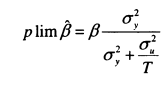
This formulation applies to both fathers and sons and has implications for estimation through both the independent and dependent variables. In the case where the dependent variable used is the true permanent income measurement, error in the explanatory variable leads to the probability limit shown below in equation (2.14); this is also true in the classical measurement error case.
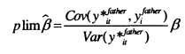

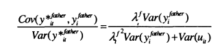
However, in this case, the variances and covariances are now functions of4, as shown in equation (2.15). This means that rather than leading to an unambiguous downward bias, measurement error in the explanatory variable can lead to upward bias if Af is <1 and Var(uit)/Var(y()is sufficiently small.

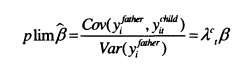
In the classical model of measurement error, error in the dependent variable does not affect the bias of the results. This result also changes if the relationship between permanent and current income varies across the lifecycle. Assuming that fathers’ incomes are measured perfectly, equation (2.16) shows that /? will be multiplied by>^f, ; there will be an upward bias if Act>l and a downward bias if Ac,< 1.

It is clear that these biases will be affected strongly by the age at which incomes are measured in the two generations. The data used for intergenerational mobility often focuses on young sons and older fathers. This combination is likely to lead to downward bias through both the dependent and explanatory variables, and possibly substantial under-estimation. To minimise the extent of measurement error, incomes for both generations should be obtained when the respective At =1 for both generations (which may be at different ages). Haider and Solon (2004) attempt to estimate this point using social security data and find that A approaches 1 at around age 42, but they do not have sufficient data to discover if this age varies across generations.
Grawe (2003) and Reville (1995) provide some empirical analysis of how estimated intergenerational persistence varies with the age of the father and son. Grawe finds strong evidence from several international datasets that measuring fathers’ eamings at older ages leads to a reduction in the estimate. He also finds more limited support for the hypothesis that estimates of p rise with the age at which sons’ eamings are measured. Reville uses data from the PS ID only, and concentrates on the age at which sons’ eamings are measured. He finds evidence that ft rises substantially with age, particularly between age 27 and 31. Reville’s evidence further supports Haider and Solon’s explanation as he shows that the rise in estimates closely tracks the eamings differential between college graduates and others at that age group. This implies that Acthlldrises as the higher educated reap the returns to their degrees.
Throughout this review I have focused on the slope coefficient (or intergenerational elasticity) as the measure of interest. In Solon’s (1992) original formulation, he couches the relationship in terms of the correlation. If the distributions of incomes are the same across generations then the correlation is equal to the slope coefficient, but if the distributions of income are not equal across generations this will not be true. In a regression which includes controls for age the partial correlation will be equal to the coefficient on father’s eamings times the ratio of the residual standard deviations.

The impact of changing variances is another way in which age affects the estimates of intergenerational mobility. The variance of income grows throughout the lifecycle, so if sons are observed at a younger age than their fathers, the variance of fathers’ eamings will exceed sons’; consequently ft will be an underestimate of the partial correlation, r.
Many developed countries have experienced strong increases in income inequality since the 1970s (see Gottschalk and Smeeding, 1997). Putting aside lifecycle effects, it is therefore likely that the variance of sons will have increased compared to their fathers; this would lead to a higher coefficient compared with the correlation. Both of these concerns mean that throughout my estimations I report both the elasticity and partial correlation estimates.
The interpretation of the coefficient is that it describes the proportion of fathers’ eamings that are transmitted between generations. If /? =.4 then comparing two fathers, one with double the eamings of the other, the son of the richer father will earn 40 percent more than the son of the poorer father. The absolute size of this eamings advantage will obviously depend on how wide the eamings distribution is. The partial correlation measure (r) is based on standardised distributions. A partial correlation of .4 means that if the first father earns one standard deviation more than the second father; the first son will earn .4 of a standard deviation more than the second.
As I have emphasised, the primary difficulty with measuring intergenerational mobility is the lack of information about the permanent income of fathers and sons. This has been the main theme of this section and it is returned to repeatedly in my empirical analyses. As we shall see, particularly critical issues are the time-averaging of parental income, the interpretation of /? when variances change between generations, and the age at which the incomes of parents and children are measured.
2.4 Summary of Current Findings on the Intergenerational Mobility of Sons
The methodological discussion in the previous section is extremely helpful in understanding the biases in the current literature on intergenerational mobility. In this section I use this knowledge to discuss some the empirical results generated by the literature so far. I explore these in three sections, the development of the US literature, a review of the international evidence and a review of what is known about changes in intergenerational mobility over time. The first of these enables me to explicitly show how methodological innovations have affected the understanding of intergenerational mobility, while the second and third sections provide a background to the questions considered in Chapters 3 and 4, respectively.
The Evolution of the US Literature
Due to the difficulties of collecting good, representative data on the permanent incomes of parents and children, many of the early studies of intergenerational mobility for the US yield low estimates of the extent of intergenerational mobility. When Gary Becker and Nigel Tomes were writing in 1986, the literature indicated estimates of around .2, from this they conclude that “aside from families victimized by discrimination, regression to the mean in eamings in the United States and other rich countries appears to be rapid” (Becker and Tomes, 1986, p.S32).
Table 2.1 provides a breakdown of a selection of papers on intergenerational mobility in the US, to illustrate how this literature has developed. Behrman and Taubman (1985) is an example of the early literature as discussed by Becker and Tomes. The sample is based on an unusual and homogenous sampling frame; the fathers are white twins who served in the armed forces. Also, the measure of fathers’ eamings is based on a single year. The intergenerational elasticity observed in this data is low, at just .23, implying that fathers pass 23 percent of their eamings advantage on to their sons.
Next in the Table is Solon’s (1992) study. This uses data from the Panel Study of Income Dynamics, which began with a national probability sample in 1968 and followed the original sample members into new households. This means that Solon is able to use information on fathers’ eamings when young men are at home in the late 1960s and early 1970s, and obtain information about sons’ eamings in the last year of data available, 1986. When a five-year average of fathers’ eamings is used as the explanatory variable, is .41.
The other results reported in the paper suggest that the use of a nationally representative sample has more impact on the results than using the five-year average of father’s eamings. When a single year of fathers’ eamings is used, estimates of /? vary between .29 and .41; already considerably larger than the .2 discussed by Becker and Tomes (1986). In order to explore the implications of sample homogeneity, Solon restricts the sample to just those sons who complete high school, the estimates using father’s 1967 eamings fall from .39 to .26 when the sample is restricted in this way.
Zimmerman (1992) uses data from the National Longitudinal Surveys (NLS) and his results confirm many of Solon’s findings. The original National Longitudinal Surveys ran from 1966 to 1981 and captured several groups; including ‘Mature Men’ and ‘Young Men’, fortunately 896 of those in the ‘Mature Men’ sample could be matched with their ‘Young Men’ sons. Fathers’ eamings are obtained from the early years of the survey while the sons’ eamings are obtained from the later years. Zimmerman experiments with averaging fathers’ eamings by up to four years, and obtains an estimate of the intergenerational elasticity of .54, even higher than obtained by Solon.
Both Solon and Zimmerman experiment with IV techniques, and I also report these results in Table 2.1. In Solon (1992), father’s years of education is used as an instrument for his permanent eamings, this leads to a higher elasticity of .53. Zimmerman (1992) uses social status measured by the Duncan Index. Using this instrument increases the coefficient on father’s 1967 eamings in a regression of sons’ 1981 eamings from an estimate of .54 using the four-year average of income, to .67 in the IV model.
The final set of results reported in this Table is the estimates from Mazumder (2001). This paper averages father’s income over a very long period in order to get close to a true measure of lifetime income. Mazumder uses a matched social security dataset and averages father’s eamings over 16 years. This leads to a high estimate of around .6. However, the top-coding of his data means that substantial imputation is made by race and education group. This is, in effect, a form of IV estimation and may lead to an upward bias on the estimates.
This summary has made it clear that taking account of methodological improvements has led to a change in the consensus about intergenerational persistence in the US. In contrast to Becker and Tomes’ reading of the literature that P was around .2, Solon’s 1999 summary states that “All, in all .4 or a bit higher…seems a reasonable guess of the intergenerational elasticity in long-run eamings for men in the United States.” (p. 1784)
Comparing International Estimates
In Chapter 3 I present new estimates of intergenerational mobility for Canada, the UK, the US and West Germany. My discussion so far has highlighted the importance played by methodology in establishing good estimates of intergenerational mobility. One of the main focuses of my empirical work on this topic is to ensure that the methodologies used are as comparable as possible. In this section I motivate my own analysis by discussing a selection of papers which measure intergenerational mobility in countries other than the US. I present the studies which have been carried out for one or two countries in Table 2.2 (many of which were also reviewed in Solon, 2002) before discussing papers which have explicitly tried to conduct international comparisons across many nations.
The papers outlined in Table 2.2 consider mobility in Canada, West Germany, Sweden, Finland and the UK. Studies have also been carried out on developing countries, but I restrict my discussion to developed countries to focus on the results most relevant to my own work .
If the consensus estimate in the US is “.4 or a bit higher” then a first glance at the evidence presented in Table 2.2 suggests that this is at the high end of the spectrum, although the UK also appears to have strong intergenerational income persistence. The studies indicate lower mobility in the Nordic countries and Canada, while mobility for Germany falls in the middle.
In the second-to-last column of Table 2 .2 ,1 indicate the approach taken to measurement error in each study. As we have seen, this can be crucial, and means that we may be reluctant to compare studies which are not comparable on this basis. Both Couch and Dunn (1997) and Bjorklund and Jantii (1997) are explicit in their desire to produce estimates for their chosen countries (Germany and Sweden respectively) which are comparable with those they produce for the US.
Couch and Dunn (1997) compare estimates from the Panel Survey of Income Dynamics (PSID) and the German Socio-Economic Panel (GSOEP). The results of this exercise produce very low, but quantitatively similar, estimates of the intergenerational elasticity of eamings between fathers and sons of .11 for Germany and .13 for the US. These low estimates are likely to be a consequence of the young ages at which sons’ eamings are measured in both countries. My earlier discussion of Haider and Solon (2004) has demonstrated that estimates obtained at young ages tend to be downward biased; but it is less clear whether the extent of lifecycle bias will be equal across the two countries. Wiegand (1997) shows that when later eamings data are used for West Germany, the measured elasticity rises substantially to around .25, so comparing single country studies indicates that mobility is higher in West Germany than in the US.
At the time when Bjorklund and Jantti (1997) were putting together their study there was no data available for Sweden which included the incomes of two generations. They overcome this by using a two-sample instrumental variables approach. They have matched information on sons’ eamings and fathers’ education for Sweden, but no information on fathers’ eamings. Fathers’ eamings during the child’s teenage years are predicted using information on the relationship between eamings and education from another dataset. Sons’ eamings are then regressed upon this prediction. Subject to certain assumptions, this estimator will be upward biased in the same way as other IV estimators. Therefore, to draw comparisons with the US, Bjorklund and Jantti repeat Solon’s (1992) PSID analysis to be comparable with their Swedish data. The elasticities from this approach are .28 for Sweden compared with .42 for the US.
Bjorklund and Jantti (1997) provide the first evidence that mobility in Scandinavian is higher than in the US. In Table 2.2 I also include results from Osterbacka (2001) using Finnish census data. This study relies on just two years of father’s eamings and shows a very low, but precisely estimated elasticity of .13. The picture of high mobility in the Scandinavian countries is confirmed by Bratberg et al’s (2004) study of Norway (which I shall discuss in more detail in the next section) and by the preliminary results from the intergenerational comparisons in Bjorklund et al (2004).
Results from Canada using matched tax data (Corak and Heisz, 1999) also indicate high mobility, with elasticities of .23, closer to the .2 of the early US analyses than the more recent literature. There may be a concern that conclusions on Canada are reliant on a single dataset but it is difficult to find a methodological reason why the US and Canadian results differ so much. Estimates are based on five year averages of fathers’ annual eamings and the authors go to some lengths to show that the data is representative.
The knowledge on intergenerational mobility in the UK is summarised by the entries in the Table for Atkinson (1981) and Dearden, Machin and Reed (1997). We may worry about the limitations of Atkinson’s data as all the fathers were resident in York and only a single week’s information on eamings was collected. Both of these aspects tend to lead to downward biased estimates. Nonetheless, the estimate of ft is high by international standards at .36. Dearden, Machin and Reed (1997) attempt to overcome measurement error problems by using a variety of techniques, as discussed above. The results vary, but in general are quite high, with the elasticity between fathers and sons at .58 when father’s education and social class are used as instruments. On the basis of this evidence it seems reasonable to conclude that in the US and UK mobility is limited compared with other countries.
As stressed by Solon (2002) methodological differences mean that it is difficult to draw firm conclusions based on a comparison of studies of one or two countries. Grawe (2004b) attempts to be more systematic. In this study, Grawe computes average and quantile regression measures of mobility for many countries, including several for developing countries. Grawe’s emphasis is on the quantile regression results which allow mobility estimates to be derived for different points of the sons’ distribution. Depending on the data available, Grawe uses a mix of OLS, IV and two-stage IV; although this has benefits in terms of bringing many datasets into play, we may continue to worry about comparability. > Grawe’s solution to this is to make only pair-wise comparisons based on the country of interest compared with results from the same estimation approach for the US. Grawe’s conclusions are that any differences found between the results from the developed countries pale into insignificance compared with those between developing and developed countries. In Ecuador, it is not possible to reject the hypothesis that the intergenerational elasticity is greater than 1.
Corak (2004) provides a review of the international evidence, but unlike Solon (2002), makes some assumptions to enable stronger conclusions to be drawn from the current literature. Building upon Grawe’s approach, Corak attempts to account for the biases introduced by different methodologies by studying how results from different approaches vary for the US (the country for which the most estimates are available). The author then scales his preferred estimates from other countries up or down depending on the likely biases. This scaling takes account of many of aspects I have shown to be important; the father’s age when his eamings are observed, the number of years used to generate the fathers’ eamings variable, and whether the estimate relied on IV methods or not.
On the basis his assumptions, Corak concludes that for the UK and US /?is around .5, for France .4, for Germany and Sweden .3 and that Canada and the other Nordic countries have /3s of around .2. This summary is not inconsistent with the conclusions I derived from my review of the literature in Table 2.2. However, concerns may remain as to whether Corak’s assumptions reasonably account for the differences in methodology between the articles he reviews. In particular, the results reported adjust only slightly for the upward bias resulting from the use of instrumental variables, as a consequence estimates from France, Sweden and the UK may be inflated compared to those from other countries6.
The studies reviewed in this section have indicated that the US, UK and France appear to have the highest levels of intergenerational income inequality (of developed countries) while the Scandinavian countries and Canada appear rather mobile by comparison. However, worries remain that these results may in part owe to differences in the methodologies used. Chapter 3 will provide additional evidence on international comparisons for some of these countries based upon explicit attempts at comparability. As a consequence, I will provide new evidence on the correct interpretation of the current literature, providing new evidence to go alongside Corak’s (2004) analysis.
6 Solon’s (1992) and Zimmerman’s (1992) results imply that IV estimates are upward biased by 25%, but the Swedish TSIV results from Bjorklund and Jantti (1997) are adjusted only from .27 to .26 to take account of this.
Evidence on Changes in Intergenerational Mobility for Sons
In Table 2.3 I review a number of papers which investigate changes over time in intergenerational mobility. The majority of studies which have looked at changes have focused on the US, with fewer looking at other countries.
One of the contributions made by Chapter 4 is to explore the way that taking alternative approaches to the data alters the results on changes in mobility for the US; so I save more extensive comments on the methodologies used in the US papers until then. The results from Mayer and Lopoo (forthcoming), Corcoran (2001) and Fertig (2002), all based on the PS ID, appear to indicate a rise in mobility in the US. Apparently, parental income has become less strongly associated with outcomes for sons. Levine and Mazumder (2002) broaden the study of changes in intergenerational mobility by adding data from the NLS and the General Social Surveys; different conclusions are drawn from these datasets, but neither is ideal for the purpose. Using the PSID once more, Lee and Solon (2004) take a slightly different approach from the other studies, using all the observations available on individuals to increase the effective sample size. They find no evidence of a change in intergenerational mobility.
Studies of changes in intergenerational mobility have also been carried out in other countries. Ermisch and Francesconi (2004) have measured changes in social mobility in the UK using occupation-based indices. They find that the intergenerational connection between occupational status has declined over time. Fortin and Lefebvre (1998) use a two-step approach similar to Bjorklund and Jantii (1997) to look at how mobility has changed in Canada for adults in the General Social Surveys of 1986 and 1994; they find no clear trend.
Two studies of changes over time have been carried for Nordic countries. The analysis presented in Bratberg et al (2004) for Norway compares intergenerational elasticities estimated when individuals are in their early 30s for the 1950 and 1960 cohorts. The authors find a slight decline in intergenerational associations for sons. Osterbacka (2004) considers this question for Finland, and finds no clear trend. Both Bratberg et al (2004) and Osterbacka (2004) confirm the impression that income persistence is particularly low in Scandinavia; the estimates from Bratberg are in the region of .15, although there is evidence that they rise to around .22 when obtained at age 45, again showing evidence of lifecycle bias.
Taken together, the evidence from the current research on intergenerational mobility points to an increase in mobility over time. In Chapter 4, I revisit the evidence for changes in intergenerational mobility in the US and
provide new results on changes in intergenerational mobility in the UK.
2.5 Theoretical Background to Assortative Mating and Family Income Persistence
In the latter part of this thesis I bring children’s partners into my analysis and model the relationship between sons’ and daughters’ family incomes and their parental income. A motivation behind this investigation is that the intergenerational persistence of family income is closer to a measure of the extent to which welfare is correlated across generations. As partner’s eamings contribute to the child’s family income the extent of intergenerational persistence is dependent upon how closely partner’s eamings are associated with an individual’s family background. This, in turn will be related to the extent of assortative mating; if couples match closely on traits which are correlated with their parents’ incomes, links between partners and parents-in-laws will result.
While the literature on this topic is much less developed than the research I have outlined on individual mobility, there are a number of theoretical papers which set the scene for the research I undertake here, and I outline these below. I begin first with the literature on assortative mating and then show the implications of assortative mating for intergenerational mobility. There are clear difficulties with measuring the contribution of assortative mating to intergenerational persistence. Many of the crucial variables are unobservable or, at least, unobserved for some of the population. I touch on these difficulties before closing this chapter with a survey of the limited empirical work that has already been undertaken on this topic.
Sociologists have traditionally dominated research on marriage and a focus of their work has been the investigation of the extent to which characteristics influence who marries who. The main aspects explored in thisliterature are marriage within and between racial, religious and socioeconomic groups; in all cases individuals tend to marry individuals like themselves. In a recent review of this literature, Kalmijn (1998) underlines three hypotheses which result in positive assortative matching: the preferences of the partners, the intervention of ‘third parties’ (such as parents) and the way the marriage market operates, which governs who individuals meet when they are ready to marry. As we shall see, the economic approach to assortative mating tends to emphasise the importance of individual preferences, but the formulation of my empirical work is sufficiently general that there is room for groups and institutions to have an impact.
The early mathematical models of marital sorting were based on assignment models. The idea is akin to all singles being placed in a room together and then leaving at the end of the evening paired-off forever. In Gale and Shapely (1962) individuals have a single ranking of partners which is common to all in the marriage market. In this case, a pure sorting equilibrium will result – the nth ranked woman and the nth ranked man will be matched, and so on throughout the distribution.
Becker’s model (1973, 1974) has a richer description of the benefits of marriage and is more strongly rooted in economic theory. For Becker, all potential marriages have an output Z. Z includes the eamings of both partners, the gains from the division of labour within marriage, as well as the utility from rearing children and from receiving affection within the family. In a utility maximising framework, all individuals will be seeking the marriage with the highest possible Z. In a sorting model with no frictions, pareto efficiency will mean that men and women will sort into partnerships which maximise the total amount of Z. The mathematical properties of submodularity and supermodularity state that output is maximised if ‘likes’ are matched when male and female traits ( Ah andA^,) are complements in producing Z.

‘Unlikes’ are matched when male and female traits are substitutes in producing Z.

From this follows the prediction that couples will be positively matched on characteristics like education and ability that are complements in the production of high quality children and negatively matched on wage rates as these are substitutes in the production of market goods. Of course, the strong correlation between education, ability and wages, means that it would be very difficult to separately identify a negative relationship between the wage rates of couples. Moreover, Lam (1988) argues that in the presence of household public goods, wage rates should be positively correlated, even conditional on other characteristics.
Recent papers have developed Becker’s model of the marriage market in search-theoretic terms. It is quite clear that in reality marriage allocations are not frictionless, it takes time to meet a partner and search is not costless. Burdett and Coles (1997, 1999) and Shimer and Smith (2000) all explore the implications of uncertainty and search costs for the marriage market. Different assumptions about the nature of the output from marriage and the way that utility is shared within couples lead to different implications for assortative mating. But in general, assortative mating is still positive in these models with frictions, albeit somewhat weaker than in the assignment models. A particular focus of the marital search literature is on modelling divorce, and I shall return to this in Chapter 7.
Chadwick and Solon (2002) provide a simple exposition of the relationship between assortative mating and intergenerational mobility, and I adopt this as a starting point for my discussion of the theoretical relationship between assortative mating and intergenerational mobility. Abstracting from the nuances of assortative mating, assume that married couples are positively correlated on the basis of their permanent incom es/*, where subscript w indicates the wife’s income and subscript h indicates the husband’s income.
![]()

Permanent incomes are transmitted according to the intergenerational relationship that has been discussed throughout, so that for wives
![]()

The combination of these two equations leads to a link between husband’s permanent income and his wife’s parents’ permanent income. This will simply be
![]()

It is therefore clear that assortative mating leads directly to a correlation between the incomes of parents and their children’s partners.
Ermisch, Francesconi and Siedler (2004) explore similar issues for the UK and Germany. To motivate their analysis, Ermisch et al use a Becker-Tomes style model to work through the implications of assortative mating for intergenerational investments and the links between incomes of different household members (putting to one side the fact that they actually measure occupational status). Unlike Solon and Chadwick, Ermisch et al assume that assortative mating occurs on the basis of human capital7 rather than permanent income, so that:
![]()

Incomes for both husbands and wives are increasing with human capital, albeit with different rates of return, ylw and ylh.

The parental utility function is a modified version of equation (2.2) which takes account of the partner’s income in the utility function as well as the son or daughter’s own income.
![]()

The parental budget constraint is binding; parents can neither borrow nor leave bequests. In this case the solution of the utility maximisation problem is straightforward; parents invest the proportion n f pH of their income in the human

capital of their children, where p H is the price of human capital. This means that the relationship between the income of parents and daughters is expressed in equation (2.27)
![]()

And the relationship between parents and the son-in-law’s income is:
![]()

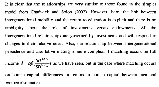

Lam and Schoeni (1993, 1994) also provide a model of the links between in-laws across generations. The focus in their papers is the relationships between the son’s eamings and his father’s and father-in-law’s education. The motivation for this model is different from the Ermisch et al and Chadwick-Solon models; rather than being concerned with what these relationships tell us about intergenerational mobility, Lam and Schoeni explore the information these relationships can provide about sons’ characteristics. They show that the effects of father’s education on wages can be interpreted as representing the impact of inherited characteristics while the effect of father-in-law’s education is correlated with uninherited attributes through assortative mating.
In Lam and Schoeni’s model the relationship between parental education and son’s eamings is driven by the inherited components of schooling, ability and wealth. Consequently, when son’s own schooling is controlled for in a regression of son’s income on father’s education, the coefficient on father’s education will fall. In the presence of strong assortative mating, controlling for the son’s education when modelling the relationship between his income and his father-inlaw’s education will not reduce the coefficient on father-in-law’s education by very much. This is because father-in-law’s schooling will be correlated with all the uninherited components of son’s income through assortative mating; it will be much more orthogonal to the son’s education than father’s education will be. Below, in the summary of results, I shall discuss the results of this exercise for both the US and Brazil, and the conclusions drawn by the authors.
The models discussed so far show links between parents and their children’s partners as an indirect consequence of marital sorting, and this type of model underlies my approach in this thesis. However, Fernandez et al (2004) propose an interesting alternative argument in the context of a son’s mother’s work status and the work status of his partner. Fernandez and her co-authors find convincing support for a direct positive relationship between a man’s mother working during his childhood and the probability of his wife working. Two possible mechanisms are posited; either men with working mothers prefer to marry women who work; or women who work prefer to marry men with working mothers, perhaps because they are more understanding and take a greater role in household work.
2.6 Measuring the Contribution of Assortative Mating to Intergenerational Persistence
Intergenerational relationships which take account of the relationship between parents and their children’s partners face exactly the same measurement difficulties as the standard relationships between parents and sons. It is important to obtain good measures of parental status for the explanatory variable, and to ensure that the measure of the child’s partner’s income is not a biased measure of their permanent income. The usual methods apply when taking account of the first difficulty, but the second becomes increasingly problematic when married women are a focus of the empirical work because of women’s more complex labour supply decisions.
The difficulties of measuring intergenerational persistence for daughters and daughters-in-law are clear. Both and 8 are based on concepts of full income, which are frequently missing in the data. Minicozzi (2002) attempts to tackle this problem head on, by making assumptions about the relationships between current income and full income for women. Minicozzi’s aim is to generate bounds on the estimated /? for daughters. However, the bounds that result are wide, from .12 to .53.
Both the Chadwick and Solon (2002) and Lam and Schoeni papers (1994) focus on the relationship between fathers-in-law’s and daughters husbands’ incomes. The obvious advantage of this is that husbands’ incomes will be closer to full income than daughters’ incomes will be. Solon and Chadwick nonetheless still use daughter’s current income in their empirical work, albeit indirectly. They show that the relationship between husband’s and wife’s combined income, and parental income (measured by the coefficient p ) can be decomposed, allowing us to get indirectly at the relationship between and 8 .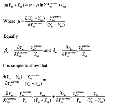

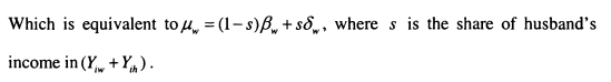

The log of the couples combined incomes can be written as

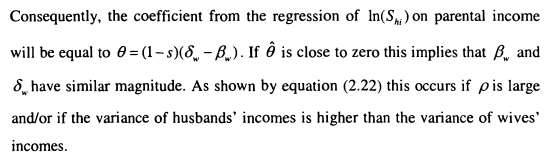

Ermisch et al (2004) estimate S and ft for both men and women. In their data they only have eamings available for Germany, so they estimate and S on the basis of occupational indices for both countries and on the basis of eamings for Germany. The use of occupational indices may overcome some of the measurement problems faced when trying to estimate concepts which require knowledge of the full incomes of daughters. While the prestige index will not be available for those not in employment, occupational status will not be affected by current hours decisions in the way that annual eamings are.
2.7 Results from the Intergenerational Mobility and Assortative Mating Literature
Table 2.4 summarises the results from several papers that take account of children’s household formation and assortative matching for intergenerational persistence.
I show an overview of the results for the three papers reviewed in the theory section; Chadwick and Solon (2002), Ermisch et al (2004), and Lam and Schoeni (1994) plus some estimates from Atkinson et al (1993) and Altonji and Dunn (1991) which offer less complete treatments of this question. The main feature to note from Table 2.4 is that the in-law’s relationship is strong in every case. In no case is the parent to son-in-law/daughter-in-law’s elasticity substantially below the parent to son or daughter elasticity, and all the in-law relationships are statistically significant. This indicates considerable assortative mating in all the countries shown here: the US, the UK, Brazil and Germany.
As we have seen, the theoretical models of intergenerational mobility emphasise that it is possible for the in-law relationship to be stronger than the relationship between parents and their own child. This is the case in two of the studies considered here; for Brazil in Lam and Schoeni (1994) and for the UK in Atkinson et al. In addition, Lam and Schoeni show that father-in-law’s education will have more information about son’s unobserved ability if assortative mating is strong; it will be more orthogonal to son’s schooling. In Brazil, this is clearly the case, adding own schooling to the wage equation reduces the coefficient on father’s education by more than it does the coefficient on father-in-law’s education in Brazil. This is not the case in the US.
Both of these pieces of evidence indicate that assortative mating is strong in Brazil. The results from Atkinson et al indicate that it also likely to be strong in the UK, while results based on occupation from Ermisch et al (2004) indicate weaker assortative mating, as 8 < for both men and women. This causes us to speculate on how contemporary results based on income will look for the UK; a question explored in Chapter 6.
2.8 Conclusion
The objective of this chapter has been to highlight the main approaches taken to the theory and measurement of intergenerational mobility and to review the empirical literature most relevant to the analyses that follow.
A number of important themes have emerged, some of which will be returned to repeatedly in subsequent chapters. As my thesis is primarily empirical, the most crucial insights discussed here have been methodological. The perfect datasets for measuring intergenerational mobility would include the lifetime incomes of two generations. My discussion of measurement methodologies has provided a number of lessons to incorporate as I (inevitably) use second best data to examine intergenerational mobility.
In the theoretical sections of this chapter I provide an economic foundation for my interest in intergenerational transmissions. I develop arguments to show how economic models of investment can explain the transmission of economic status between generations. I have also shown, however, that it is difficult to distinguish models of intergenerational investment from persistence resulting purely from inherited characteristics. The role of human capital is important in whichever model is used, and I explore the extent to which differences in education are responsible for intergenerational inequality in several of my studies.

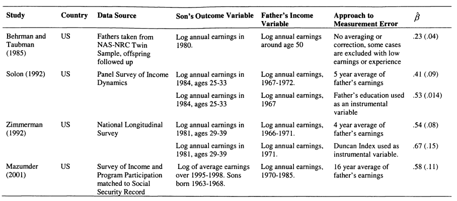

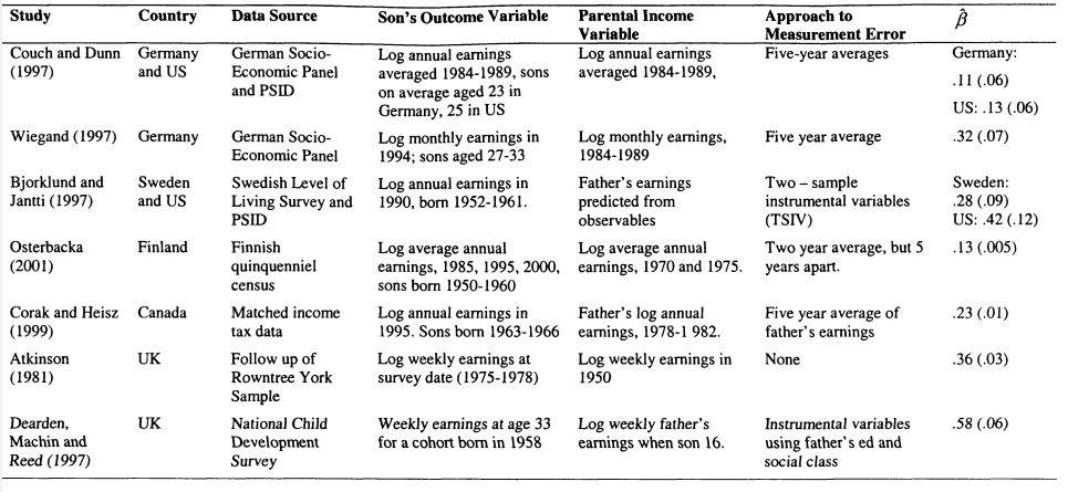

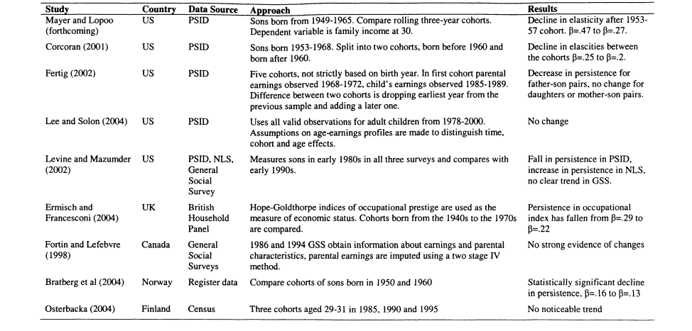

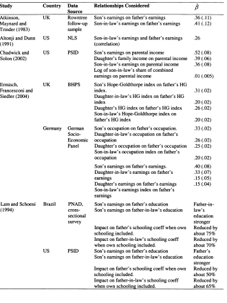
Chapter 3: International Evidence on Intergenerational Mobility8
3.1 Introduction
The early literature on intergenerational mobility suffered from interpretation difficulties; it was unclear the extent to which a particular estimate of the intergenerational elasticity (say .4) constituted an indication of a large or small amount of mobility. An important way in which this question has been illuminated has been through making comparisons of the extent of intergenerational mobility across countries. In addition, such comparisons can lead to an understanding of the economic mechanisms that lie behind variations in levels of mobility for different places.
Comparisons are made problematic, however, by the lack of truly equivalent estimates found in the literature. Different researchers take their own decisions about variable choice, sample selection and estimation methods, meaning that it is impossible to know whether variations are a consequence of fundamentals, or a lack of comparability. The review of the measurement of intergenerational mobility provided in Chapter 2 has emphasised the biases which result from using imperfect data to measure intergenerational mobility. It has also highlighted the fact that perfect data is almost impossible to come by. All estimates of intergenerational mobility are likely to be biased to some extent. The strategy with estimating internationally comparable estimates of intergenerational persistence is to ensure that biases are similar across countries. In this chapter I attempt to add to the literature with some really careful estimates of intergenerational mobility for males in the UK, the US, Canada and West Germany.
The discussion in Chapter 2 encourages us to worry about a number of aspects of estimation which can lead to potential biases. First and foremost there is the difficulty of measurement error: all measures of parental income are likely to be imperfect measures of parents’ permanent income, so it necessary to take steps to ensure that the bias is not worse in some countries than others. Second, is the problem of lifecycle measurement error, as highlighted by Haider and Solon (2004). The obvious solution to this problem is to ensure that parents’ and
8 This chapter was supported by funding from the Sutton Trust. I would like to thank Joan Wilson for research assistance with the GSOEP data.
children’s incomes are observed at similar ages across datasets, but as I shall show below this may not suffice. In addition, it is of course important to assume that the variables used are measuring the same concepts across countries, and that the samples are similarly selected.
Chapter 2 provided a review of the international evidence on the intergenerational mobility of sons. The conclusion which emerges from the literature so far is that mobility appears to be more limited for the US, UK and France, with Sweden and West Germany exhibiting moderate mobility and Canada and the remaining Nordic countries being most mobile. What is also illustrated in Chapter 2 is that comparisons made on the basis of the existing literature may not be satisfactory. In many cases estimates are drawn from single country studies and take no account of the importance of common methodology. While Corak’s (2004) meta-analysis takes into account the way in which methodology will affect the estimates, we may wish to verify his results as they rest on strong assumptions about the extent of the biases introduced by different measurement approaches.
It is clear that the literature would benefit from a more systematic approach to comparisons across countries. The results reported here are crosssectional comparisons of mobility for young men in the UK, US, Germany and Canada bom around 1970. The datasets used are the British Cohort Study, the PSID, the GSOEP and the Canadian Intergenerational Income Data respectively. All of these studies have been used in intergenerational analysis previously. Comparisons of single country studies (ie Solon 1989, 1992, Dearden et al 1997, Wiegand, 1997 and Corak and Heisz 1999) encourage us to expect that mobility is lower in the US and UK, and higher in Canada and Germany. My results generally confirm this picture. Income persistence is strongest in the US and UK, with moderate persistence in Germany and more mobility in Canada. Unfortunately, due to small sample sizes, the only significant result is that there is more mobility in Canada than in the US and UK.
As well as providing more information to evaluate levels of intergenerational mobility across countries “comparisons of intergenerational mobility across countries may yield valuable clues about how income status is transmitted across generations and why the strength of that intergenerational transmission varies across countries.” (Solon, 2002, page 59, original emphasis). My discussion, in Chapter 2, of Solon’s (2004) model of how intergenerational mobility varies across time and place, showed that the relationship between parental income and son’s human capital and the returns to human capital both have crucial parts to play in the transmission of economic status between generations.
In order to find out how the contribution of education to intergenerational persistence varies across countries, I decompose my estimates of the intergenerational elasticity into three parts; the part due to return to education, the part due to educational inequality and the part unexplained by education. My estimations show that education is important in generating earnings persistence in all countries, but particularly so for the US, due to high earnings returns to education.
This chapter proceeds in the next section by describing my empirical approach followed by a description of the data in Section 3.3. Section 3.4 discusses the results for the comparison of intergenerational mobility; Section 3.5 describes the decompositions, while Section 3.6 concludes.
3.2 Empirical Approach
The majority of this chapter takes a standard regression approach to measuring intergenerational mobility, where the parameter of interest is /? from the regression of sons’ earnings on parental income for individual i in country j.
![]()

In my estimations I use earnings at around 30 years old and parental income at around age 16. The choice of comparable ages is motivated by Haider and Solon (2004) and Grawe’s (2003) observations about lifecycle bias, an issue to which I return below.
The mainstream intergenerational literature has concentrated on measuring the elasticity between fathers’ earnings and sons’ earnings. However the British dataset does not have separate measures of father’s earnings, so I use parental income instead. This seems to be an equally interesting measure and makes sense from an investment point of view, as I am able to see the impact of total resources in childhood. Also, I do not lose as many observations due to missing fathers. I supplement the analysis with measures of father-son elasticity where possible, to improve comparability with the existing literature. The difference between measures of mobility based on parental income and those based on father’s earnings is obviously related to the extent of lone parenthood in the countries and female participation in the countries under discussion; I shall return to this point in the results section.
To take account of variations in the income distributions between the two generations I also report the partial correlation between parents and sons’ incomes, r. In a regression which includes controls for age, the partial correlation will be equal to the coefficient on father’s earnings times the ratio of the residual standard deviations. I report this as an alternative measure of persistence.
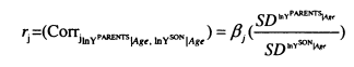

The advantage of this measure is that it is insensitive to differences in the variance of sons’ and parents’ incomes within the sample. This is an issue for three reasons: first, as pointed out by Grawe (2003), the variance in parental income is likely to be larger because parents are further along in their lifecycle – this will reduce p , this will be compounded in this case by measuring income for parents but earnings for sons. In terms of comparisons over countries, different lifecycle patterns of income and earnings variance could lead to different estimates of P but will not affect r. The correlation measure of mobility also takes into account the different levels of inequality between generations and changes in inequality between generations and over time. This may prove to be particularly important as I am considering mobility for young men growing up as inequality rose considerably in the US and UK, and more moderately in Canada and West Germany (see Gottschalk and Smeeding, 1997, Table 4).
In Chapter 2 I stressed the importance of using nationally representative samples and minimising measurement error, illustrating how early estimates of intergenerational mobility were substantially biased downwards due to these issues. The first of these concerns hopefully should not be relevant here, as all the data sources used here should be broadly representative of the population.9 Measurement error is more of a concern, and to overcome it, I average income over a number of years wherever possible. My approach is discussed in detail below when each country is taken in turn.
In addition to the regression results, I present some estimates of transition matrices. These are derived by dividing the income distributions of parents and children into equal numbers of quantile groups (I use quartiles) and noting the proportion from each parental quartile which finish in each quartile of the children’s distribution. Complete immobility is represented by all of the children who begin in a particular quartile remaining in the same quartile (all cells in the leading diagonal equal one, the others equal zero), complete mobility would be where the starting quartile has no effect on the destination (all cells equal .25). An index of immobility is generated by adding the values found in the lead diagonal and adjacent cells.
To consider the role of education in underpinning intergenerational persistence I borrow a considerably simplified version of Solon’s (2004) model. It is clear that education attainment varies according to parental income, such that Ed*™ = a0j + y/j In YijH,rent* + etJ. This is due to both differing endowments and differing investments across families. Education has benefits in the labour market such that In Y*™* +aXj +<pjEd*°ns +u(Jwhere (f>j denotes the return to education in country j. This means that the overall intergenerational elasticity can be decomposed into the return to education multiplied by the relationship between parental income and education, plus the unexplained persistence in income that is not transmitted through education.
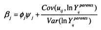

The data available only allows education to be measured by quantity (and even this is done crudely, as discussed in the data section) so aspects of the quality of education, as well as many other unmeasured factors, will be included in the unexplained component.
However, the extent to which surveys are representative can be affected by attrition and this issue is discussed in the Appendix.
3.3 Data
Intergenerational Mobility Data
The UK analysis is the building block for the approach taken to the rest of the data used in this chapter. In some respects the UK has ideal datasets for exploring intergenerational relationships, as it has two large cohort studies which observe children from birth to adulthood, also obtaining information about parents along the way. I use the second of these datasets, the British Cohort Study (BCS), for comparisons of mobility across countries. The members of this cohort are all those bom in a single week in 1970; gross weekly usual parental income data (but not father’s earnings) is available for age 10 and age 16, and gross weekly usual adult earnings are collected in 2000 when individuals are 30.
In both years when parental income information is collected in the BCS, income is reported in bands rather than continuous amounts. I generate continuous variables by fitting a Singh-Maddala distribution to the data using maximum likelihood estimation. This allows me to find the expected value within the band. This is particularly helpful in allocating an appropriate value for those in the top category10.
The dataset used for the US analysis is the Panel Survey of Income Dynamics. This is an annual survey which began with 4800 families in 1968. Analysis is restricted to those young men who are children of the initial sample members (excluding the Survey of Economic Opportunity members) who were bom between 1965 and 1973. Parental income and fathers’ earnings are observed at age 16 and the four adjacent years, and sons’ earnings are observed in 2001 (and therefore refer to 2000).
The disadvantage of my precise approach to comparability is a very small sample of just 187 sons. This is to a large extent a consequence of the reduction in the core sample from 1997. Such a small sample unsurprisingly leads to rather large standard errors. In order to reduce these difficulties, I also report estimates for a larger sample of all sons bom between 1954 and 1970.1 once again observe
10 Singh and Madalla (1976). Many thanks to Christopher Crowe for providing his stata program smint.ado which fits Singh-Maddala distributions to interval data.
parental income in the years around age 16 and observe sons’ earnings for age 301 \ and this leads to a much improved sample of 527.
There are a variety of variables available to measure parental income, after experimentation I have settled on the “family money” measure less the earnings of those other than the “head” and “wife”- this is motivated by the fact that the teenager’s own earnings will be correlated with his later labour market performance. I also present results using father’s gross earnings as the explanatory variable. Both of these variables are annual amounts.
For West Germany I use the German Socio-Economic Panel, which is based on very similar principles to the PSID. Unfortunately it began much later, in 1984. As in the PSID, I select the sample of young men bom between 1965 and 1973. The short panel means that I am unable to follow the full sample from ages 1 0 14 to 18, instead I use parental income information from 1984-1988 . The parental income variable is household net monthly income; once again the teenager’s own income is subtracted. The outcome measure used is gross monthly earnings in 2000. The GSOEP consists of a number of sub-samples; I restrict to the core nationally representative sample. As with the PSID, the stringent approach to comparability leads to a small sample of around 220, so I also use a supplementary sample which includes some older sons (those bom between 1960- 1973), raising the sample to 289.
The Canadian analysis is based on information from the Canadian Longitudinal Tax Records held by Statistics Canada. The tax records provide information on all income tax returns in Canada between 1979 and 1998. Information on names, addresses and ages included in the data allowed Statistics Canada to match individuals bom between 1962 and 1970 with their parents, this was possible provided both generations filed a tax return while the child was living at home in his or her late teens.13 The matched data forms the Intergenerational Income Data (IID) and its basis on administrative records means
11 For sons who turn 31 in 2000 or 1998 (the years when there was no survey) data for the following year is used.
12 This means that the age at which family income is measured ranges from 11-15 to 19-25 and is collinear with sons’ age. This effect should be ameliorated by controlling for son’s age.
13 This requirement is less stringent than it would be in the UK as individuals are legally required to file a tax return if they worked at all in the previous year, so this will include part-time and holiday work of those in education
its size is considerable: Statistics Canada estimates that the data includes around 70 percent of the relevant age group (Cook and Demnati, 2000). A more complete description of the creation of the data is given in the appendix to Corak and Heisz (1999) and Oreopoulos (2003).
One of the main advantages of using administrative data is that there is considerably less concern about attrition and measurement error, particularly as most earnings reports come directly from the employer. The reliance on tax records brings with it a worry that the data may not be fully representative of the Canadian population. One of the key requirements to be included in the dataset is that the parent and child both file for tax while living in the same household. The dataset will therefore exclude those with no labour market attachment in their teenage years, those who leave home before they start working, or those whose parents have no labour market attachment. Evidence from Corak and Heisz indicates that the selections introduced by the matching process do not change the results.
For comparability purposes, I focus on a young group within the sample, those bom between 1967 and 1970. Sons’ gross earnings are obtained from the most recent year available, 1998. Parental income is, as with the PSID, obtained at age 16 and the surrounding four years. I use total parental income as the explanatory variable; this is market income plus pensions, grants and employment insurance. Significantly, it does not include welfare payments, as these were not required on the tax return until 1992.
In all the countries where samples include more than one son per family, I include all the sons available and cluster the standard errors by family identifier, thus accounting for the correlation between unobservables among brothers. Other studies also restrict to sons who have both parents present in the household, I do not. Consequently, I use the average age of the parents to control for differences in parents’ ages. One additional restriction is necessary. The British and Canadian data do not include self-employment income in the earnings variables; I therefore exclude the self-employed from all samples.
A focus on comparability has been at the forefront of the construction of the data used in these studies. However, there are some differences which are unavoidable. The British income data for both generations is collected on a weekly basis, whereas for Germany the income data is monthly and for the US and Canada it is annual. In Chapter 2 I emphasised the downward-biasing effect of measurement error. It is clear that weekly income is likely to be a more erroneous measure of permanent income than annual income. Unfortunately, relatively few studies have attempted to quantify the magnitude of this impact. Boheim and Jenkins (2000) consider the implications of using weekly rather than annual income measures to compute the extent of inequality using British Household Panel data. The authors find that in the distribution of income does not vary much depending on the measure used; however, this does not mean that a household’s position in the income distribution does not fluctuate. In the context of measuring intergenerational mobility, we might expect this non-comparability to bias down the estimates for the UK and Germany compared to the US and Canada. However, it should be emphasised that the information asked for in the UK is ‘usual’ weekly income, hopefully meaning that not all week-by-week fluctuations will be reported.
Education Variables
In order to decompose the intergenerational elasticities into those parts explained and unexplained by son’s education level, it is necessary to have comparable measures of continuous education across countries. Unfortunately, the Canadian tax data does not offer any information about education levels; it is therefore not possible to include Canada in this analysis. In order to believe the decompositions for the other countries, it is essential that the education variables used are comparable.
The custom of measuring educational attainment by years of schooling is quite reasonable in the US system. Young people take one grade per year and measured schooling naturally takes the form of ‘grades completed’. This measure is particularly useful as not only does it measure schooling continuously but it also has an attainment component, as students sometimes have to repeat grades in order to pass them.
The situations in the UK and West Germany are not so simple. The education systems in these two countries are clearly based on qualifications attained rather than grades completed, and students follow alternative tracks. For example, in West Germany students are split into qualitatively different schools at around age 13. In order to resolve this difficulty I convert the qualifications attained into years of schooling in the UK and West German data. In the UK this is done crudely on the basis of the usual age that individuals leave education after attaining the highest qualification recorded. In West Germany I use the schema developed by Pischke (1993) which is based on adding the years spent at school (which depends on the school type) to the years spent in vocational training (the work-experience component of apprenticeship is acknowledged by allocating half a years schooling to each year spent achieving one) and the years spent at university. The resulting coding is extremely similar to the one derived specifically for cross country comparisons by Lillard et al (2002).
Educational attainment can also be measured categorically, to better recognise the different structures of the education systems in different countries. Steedman, McIntosh and Green (2004) derive a categorisation of comparable education levels in order to conduct a cross-country comparison of skill attainment. This is a difficult task, as some qualifications do not match up well across countries. In order to overcome this difficulty Steedman et al allocate proportions of individuals with a particular qualification to different codes. This is not suitable for my micro-level analysis. Instead, I use four categories of attainment similar to the Steedman et al coding which are broadly comparable with lower secondary attainment, secondary attainment, some post-secondary schooling and higher education (more details are provided in the Appendix). While this categorical variable cannot be used to decompose the explained part of persistence, it can be used to check how the levels of returns compare across countries and to derive the unexplained part of persistence.
3.4 Comparative Measures of Mobility
Table 3.1 summarizes the samples used in my comparative estimates of intergenerational mobility for the UK, the US, Germany and Canada, and provides a survey of the information in the data section. This Table highlights my focus on individuals bom around 1970 and my aim to measure sons’ parental income when they are approximately 16 and their own earnings at around 30 years old. In addition, it shows clearly the difference between the comparable samples and the extended samples used for the US and West Germany.
In order to minimise the impact of measurement error I wish to use timeaveraged measures of parental income wherever possible. However, the extent to which this is possible varies across the surveys. In particular, in the British data income measures are only available at ages 10 and 16. I therefore present results for three different income measures: single year income, averages of income over two years and income averaged over five years.
Descriptive Statistics
Table 3.2 describes the data used in this section of the analysis. Means and standard deviations are set out for the variables used, both in levels and logs. Direct comparisons of the measures are made difficult by changes in exchange rates over time, however some issues are apparent.
The first two lines of the Table show how the mean ages of sons and parents compare between countries. These re-emphasise the focus of the samples upon sons at around age 30 to 31, although the sons from the extended West German sample are rather older, with a mean age of almost 33. The average parental age is very similar across countries at around 43-45, although parents in the UK and US appear to be somewhat younger than those in West Germany.
Moving on to the income measures, for the UK sons’ average earnings at age 30 are slightly larger than their parents’ income at age 16; in all other countries the opposite is true. Additionally it is the case that there is greater inequality in the UK in the sons’ generation than for parents, which is not the case for the other countries. This appears to indicate that measurement problems in the UK data lead to an underestimate of the mean and variance of parental income. To a certain extent the low variance found in the data is a mechanical consequence of the fact that it is based on banded data. It is difficult to know what to do about this; however the fact that the correlation is independent of relative variances Germany rather lower. After the adjustment, the gap between mobility in Canada and in the other countries increases.
The results based on two-year averages of income in the second panel are slightly higher than in panel (1). This indicates that averaging over two years of data reduces measurement error to a certain extent. The patterns are very similar to those for the single year estimates with weaker mobility exhibited in the US and UK and more mobility shown in West Germany. Unfortunately I cannot add comparable estimates for Canada to this table at present, but as we shall see, estimates using five years of data also indicate high mobility, so it is reasonable to say that mobility in Canada is high by international standards.
The five year averaged results given in the lower panel are higher in all countries as one would expect, showing that the use of a more permanent measure of income reduces measurement error. The largest change when we move from the single-year to the averaged results is for the US, where r rises from around .23-.26 to around .35-.4. This large change indicates more transitory income mobility in the US. It also raises questions about the extent to which estimates for the UK would rise if more years of data were available. Comparing across countries, the results are similar to those presented for a single measure of income, although the gap between the US relative to Canada and Germany has widened.
These results seem to broadly confirm expectations from the literature; however before taking these conclusions too far, it is important to see the extent to which it is possible to distinguish the estimates from each other when some of the samples used are so small. To consider this question, I include 95 percent level confidence intervals for all the estimates. The small sample sizes used for the US and West Germany lead to very large confidence intervals, although it is clear that the use of the extended samples reduces them somewhat. The very large sample provided by the administrative data in Canada gives us much more confidence about the level of mobility there, and I can say that mobility in Canada is significantly greater than mobility in the UK and the US.
Table 3.4 provides results for the father-son elasticity of earnings for the US, West Germany and Canada. Once more the averaged results show a higher elasticity of earnings from father to son in the US than in other countries. For West Germany the estimates of /? for father’s averaged earnings on the extended sample is .303 and r is .283. This is substantially higher than obtained by Couch and Dunn (1997) and Grawe (2004), but much more similar to the results obtained by Wiegand (1999). This increase in the estimate closes part of the gap found in Table 3.3 between the US and Germany, although persistence in the US still appears to be greater by the partial correlation measure. Once again, the pointestimates of the correlations imply that there is more mobility in Canada than in the other countries under study.
A comparison of the estimates in Table 3.4 with those reviewed in Chapter 2 generally show that the approach to the data taken here does not lead to a large change in the estimates of intergenerational mobility. An exception to this is the P for the US which is .33 based on five years of father’s earnings compared to .41 for a similar specification in Solon (1992). Although it appears substantial at first glance, this difference is not statistically significant. The difference reflects the rather small sample sizes used in intergenerational analyses of the PSID, and the sensitivity of the analyses to differences in definition and the years of data used. These features of the data are discussed more fully in Chapter 5.
The Inequality Adjustments
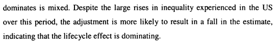


Parental Income Mobility versus Father’s Earnings Mobility
In the US and Canada /? is slightly higher for family income than for father’s earnings. This is what might be expected if total resources during childhood are more important than individual parents’ earnings; this is in line with the human capital investment model described in Chapter 2. In West Germany the reverse is true when comparing averaged results, and as we have seen, this difference is important as it reduces the gap between estimated mobility in the US and West Germay.
This difference could have several causes. In the first case it could be a consequence of sample selection; to be included in the fathers’ earnings regressions there must be a working male head of household. However, imposing this restriction on the parental income regressions does not explain any of the differences. Second, in the German data income is measured net of tax with transfer payments included, while the US data does not subtract tax, so will account for less redistribution16. If the appropriate transmission mechanism within the family is based on endowments rather than investments, more redistribution will result in less persistence from family income to son’s earnings. I have checked this hypothesis by using gross joint parental earnings; once again there is substantially less persistence in Germany than when mobility is measured using fathers’ earnings.
This leads to the conclusion that there is a genuinely stronger transmission mechanism to sons’ earnings from fathers’ earnings than from parental income in West Germany. This is confirmed by splitting the sample into families where both parents’ work and where only the father works. If father’s earnings are truly more closely linked with sons earnings then we would expect a larger association on parental income when the father is the only breadwinner. There is suggestive
16 We would expect there to be less redistribution in the US even if the data was measured
comparably.
evidence that this is the case, for the extended sample the partial correlation is .169 (.089) among families were both parents work while it is .259 (.082) for families were only the father works.
In West Germany the sole-breadwinner model lasted rather longer than in any of the other countries studied: for example Fitzenberger and Wunderlich (2002) show that the rise in employment for females in West Germany has been much smaller than in the UK. In 1986 50 percent of mothers are working in my German sample, compared with 70 percent for a comparable sample of 16-yearolds in the US. This is likely to mean that the selection of mothers into work is different and has implications for the contribution of mother’s wages to household income. These contrasts between West Germany and the US provide some suggestive evidence in favour of the importance of endowments rather than human capital investments in generating intergenerational persistence. In the investment model it should be income as a whole which determines investment; in Germany this is very clearly not the case, with a stronger relationship between fathers’ and sons’ earnings only too apparent. If assortative mating on endowments is similar for parents in the US and West Germany, then we would imagine that higher female participation leads to parental income being more closely related to parental endowments in the US, accounting for the stronger relationship between sons earnings and parental income in this country17.
The important distinction between measuring family resources by either parental income or father’s earnings has been given scant attention in a research area which began when father’s earnings and family income were more legitimately interchangeable. This is clearly no longer the case, and the results discussed here have illustrated that comparing intergenerational estimates with different explanatory variables may be able to tell us more about the mechanisms which underlie mobility. This area is clearly ripe for further research.
Transition Matrices
17 This discussion also has implications for the intergenerational mobility of women, with the implication that we would expect mobility to be higher for women compared with men in West Germany. This deserves further investigation
Tables 3.5, 3.6 and 3.7 and 3.8 show transition matrices between sons’ earnings and averaged parental income for all four countries. For the US and West Germany I use the extended samples. For the US, UK and West Germany I use two year averages of parental income and remove the age variation before dividing the data into quartiles. These transition matrices imply rather more persistence across generations for the US than for the other countries. The aggregate index of immobility is 3.092 for the US compared with 2.885 for the UK, 2.798 for West Germany and 2.771 for Canada. One of most important features of these transition matrices is the higher proportion of individuals with parents in the poorest quartile who remain in this quartile in the US; .417 compared with .374 in the UK , .322 in Canada and .304 in West Germany. There is also a higher degree of persistence at the top in the US and UK compared with the other countries, so not only is it harder to climb up, but it is also more difficult to fall down the income distribution relative to one’s parents.
Life-cycle earnings profiles
Taking on board the findings of Haider and Solon (2004) about the biases introduced by observing sons at a young age, I have been careful to observe sons at the same age in all countries, apart from in Germany where the sons in the extended sample are somewhat older. In this section, I demonstrate the importance of this restriction, the implications of relaxing it, and comment upon whether it is sufficient to ensure that estimates are truly comparable across countries.
Since Mincer (1958), it has been acknowledged that workers with more training have steeper eamings-experience profiles, and therefore that the returns to education tend to increase with age. In Haider and Solon’s formulation of measurement error, At indicates how different age-eamings profiles by skills result in current income underestimating permanent income for those with higher permanent incomes.
![]()

I explored the way that this type of measurement error introduces bias through both fathers’ and sons’ incomes in Section 2.3. These biases will lead to an underestimate of p if sons are observed at a young age when At<\. Ideally we wish to compare sons at the same point in their age-experience profile, and differences in age-eamings profiles across countries may mean that the current approach does not suffice.
Figures 3.1 to 3.4 explore age-eamings profiles for men between 25 and 38 of different education levels for all four countries; this should give an impression of the time path of At for sons in each country18. Mincer’s prediction is true in all cases with steeper earnings growth for the most educated group. In the US and Canada there appear to be higher returns to college education than in the UK, but the age profiles are similar. In West Germany however, the wages of college graduates rise much more steeply than for other groups in their early thirties and the full returns do not appear to be reaped until men are around 35. This is around 4-5 years later than in the other countries and may indicate that At = 1 at a later age. It may be, then, that this effect leads to an underestimate of P in Germany for younger sons and explains why the results for West Germany increase when I include older sons in my expanded sample19.
3.5 Decomposing Intergenerational Mobility
Finally, I turn my attention to the mechanisms which may underpin the variations I find in mobility across countries.
In order to motivate the education decompositions which follow, Table 3.9 shows a breakdown of education levels in the intergenerational samples for the UK, West Germany and the US20, both by years of schooling and by my categorical education variable. The mean number of completed years of education
18 In order to minimize the impact of the sample selections inherent in the intergenerational data, I use the Labour Force Survey for the UK, the Current Population Survey for the US, the full GSOEP for Germany and the Survey of Labour and Income Dynamics for Canada.
19 It also may explain why the estimates for young sons in Couch and Dunn (1997) are so much lower than my own.
20 From this section onwards I focus on results for the extended samples for the US and West Germany.
is broadly similar across the three countries, at around thirteen years. In all cases the distributions are bi-modal with a concentration of young people completing between 10 and 12 years, and a further concentration at 16 years. The lower part of the table indicates that the implications of different years of education for the level of qualifications vary substantially across countries. In West Germany, many students leave after 11 years of education or less; but Germany does extremely well when education is measured by qualification level, with only 7 percent of the sample achieving below level 3 in my schema. This is due to the success of West Germany in producing well-qualified apprentices who have spent relatively little time in formal schooling. In all three countries more than one fifth of the sample are graduates, with the UK performing particularly well in this regard with almost 30 percent achieving a degree.
Table 3.10 provides an analysis of the returns to education by country, using both measures of education. The return to a year of education varies substantially across countries. It is highest in the US at .106, .075 in the UK and .064 in West Germany. These results can be compared with those found by Denny, Harmon and O’Sullivan (2004) who use data from the International Adult Literacy Survey to estimate the returns to education in many countries. Their samples of all working individuals show returns to a year of education of .100 for the UK, .089 for the US and .054 for Germany. These seem broadly comparable with my findings, bearing in mind that my samples focus on a particular cohort of young men.
The second set of results in Table 3.10 present returns to qualification level. These present a rather different picture from the years of education results. Again, the returns to education in the US are higher than in the other countries; but the gap between the UK and West Germany has closed, with returns to qualifications in these two countries now appearing extremely similar. This indicates that the years of education variable for West Germany should be treated with some caution in the decompositions. This is not surprising given the descriptive patterns which showed many people attaining level 3 qualifications after a short period of schooling.
Table 3.11 shows decompositions of intergenerational mobility. These are based on the intergenerational coefficients, when two-year averages of parental income are used as the explanatory variable of interest. The estimates of P reported here imply that the UK is least mobile, followed by the US and then Germany. The partial correlations presented in Table 3.3 gave a slightly different pattern showing mobility to be weakest in the US, then the UK followed by West Germany. The difference in the ranking of the UK and US is due to the larger variance in parental income in the US, as discussed previously in the text. Either way, the large standard errors mean that the estimates are essentially indistinguishable.
The first aspect to note from the decompositions is the importance of educational levels in explaining intergenerational mobility. Differential levels of education explain between 35 and 50 percent of intergenerational mobility across countries, this is the case even when education is measured crudely by years of schooling. The largest contribution of education to intergenerational persistence is made in the US, where 50 percent of the p coefficient can be explained by my simple decomposition. In particular, the strong returns to education in the US play an important role. The UK has the highest extent of persistence in this specification, this is driven both by a relatively strong relationship between educational attainment and parental income and also by a large unexplained component. Further investigation of this unexplained component is an obvious target for future research.
As noted above, the large variance in parental income in the US leads to an underestimate of p for that country. It is clear from the parts of the decomposition shown in Table 3.11 that both the returns to education and the relationship between parental income and education (measured by the covariance) are stronger in the US, and that these lie behind the strong income persistence found in this chapter. It is possible to use these results to calculate some counterfactuals. To take two examples: if the UK had the same relationship i between education and parental income as the US , ft would equal .340, much higher than its actual level. Similarly, closing the gap in returns between West Germany and the US would lead to closure in the gap in p for the two countries; p for West Germany would be .262.
21 In calculating this counterfactual it is important to remember that both variances and covariances contribute to regression coefficients. I vary the relationship between parental income and education while keeping the variance of parental income constant.
As I have already stated, these results are strongly contingent upon us having faith in the measures of educational attainment used. Although it is not possible to do a complete decomposition using the categorical measures, these alternative measures of educational attainment can be used to make a number of comments about the decomposition results presented in Table 3.11. The results presented in Table 3.10 strongly suggest that the use of the years of education variable is underestimating the role of educational returns in generating intergenerational persistence in West Germany. This implies either that the relationship between parental income and years of schooling or that the extent of unexplained persistence is exaggerated for West Germany in Table 3.11.
To investigate the sensitivity of the results to the education measure, I recalculate unexplained persistence for all countries, using the four category education attainment variable. The change to the unexplained component is remarkably small. In the UK slightly less mobility is explained by education, with the unexplained component estimated as .184 using the education categories, compared with .177 using years of education; for the US this comparison is .138 compared with .134. In West Germany, where we might expect the strongest influence from changing the education variable, there is no difference; the new model reveals unexplained persistence to be .135 regardless of which education variable is used. This indicates that the West German results may overestimate the importance of differences in years of schooling by parental income level and underestimate the importance of the returns to education in generating intergenerational persistence.
3.6 Conclusions
This research has attempted to provide a new approach to the data sources for estimating intergenerational mobility across countries. By attempting to make the mobility estimates as comparable as possible, I illustrate some of the important methodological issues in the current literature on cross country estimates of intergenerational mobility.
This comparative study of intergenerational mobility indicates that there is somewhat more mobility in Canada than in the other countries under examination. Drawing further firm conclusions about relative mobility in the US, UK and Germany is prevented by small sample sizes. The small samples used for the GSOEP and PSID are partly a consequence of the stringent approach I take to ensuring comparability; implying a trade-off between precision and comparability. However, this is only part of the story.
One of the motivations behind this Chapter was to address the concerns about the comparability of methodology across countries in the estimates intergenerational mobility to date. It was anticipated that the results found would be able to shed light on the most important dimensions where comparability is important. In particular, I wished to evaluate surveys such as Corak (2004) that use assumptions about the impact of differences in methodology to overcome some of the non-comparability between studies of individual countries.
In general, the results from this survey have been in line with those from the literature to date. Throughout, I have emphasised that the size of the standard errors prevent me from drawing strong conclusions, this appears initally to be a disadvantage of the methodology adopted. However, it should be noted that many of the standard errors in the survey in Table 2.2 would also prevent strong conclusions being drawn from comparisons across studies. For example, there is no statistically significant difference between Solon’s (1992) .41 estimate (standard error .09) for the US and Wiegand’s (1997) estimate of .32 (standard error .07). The statistical significance of Corak’s (2004) conclusions will be affected not only by the precision of the estimates in the original study but also by uncertainty over the assumptions made to overcome methodological differences. In fact, Corak does not include any standard errors in his review. Consequently, while the point estimates found in this chapter may not be dramatically different from those found in across country studies, an advantage of the methodology adopted here is the explicit consideration of the uncertainty inherent in cross country comparisons of mobility.
Putting aside these caveats, point estimates of the elasticities appear to indicate somewhat less mobility in the US and UK, with West Germany more mobile. In the last Section of the Chapter measurement questions were put aside to address the more interesting question of why mobility varies across countries. Many models of intergenerational mobility stress the role of education in determining the persistence of incomes across generations. My explorations for the US, the UK and West Germany indicate that this is important, with higher returns to education being particularly crucial in driving the low mobility found in the US, while a strong relationship between parental income and education is a feature for the US and the UK.

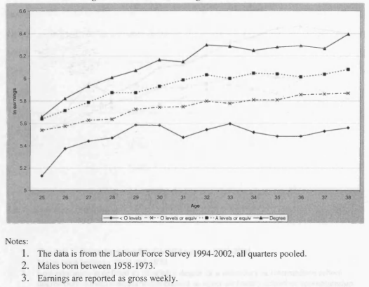


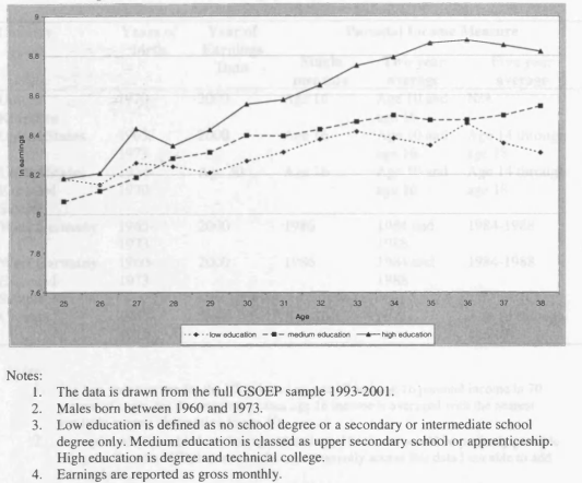
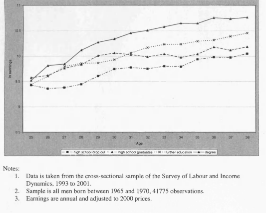


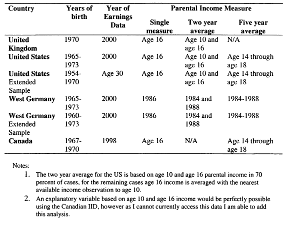

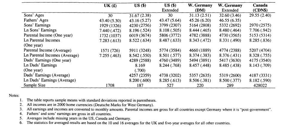

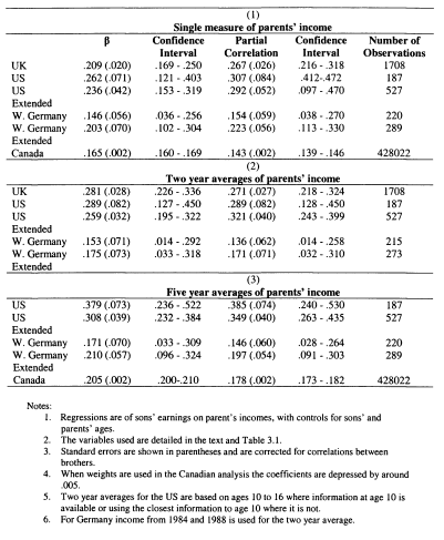
Mobility Based on Parental Income

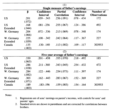
Based on Fathers’ Earnings

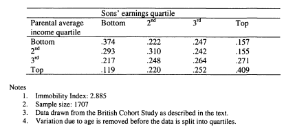

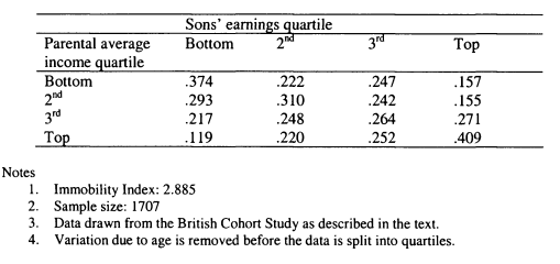

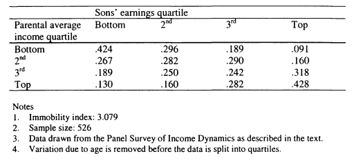

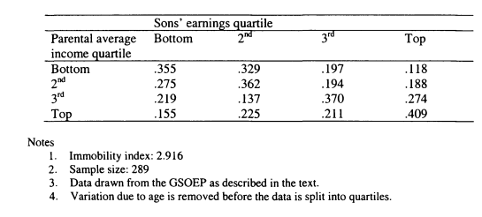

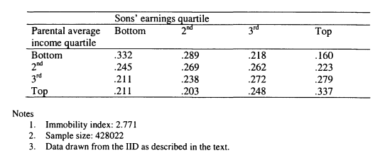

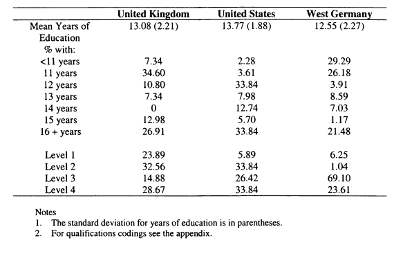

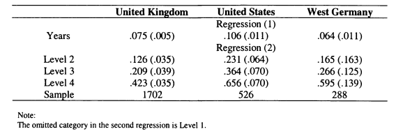

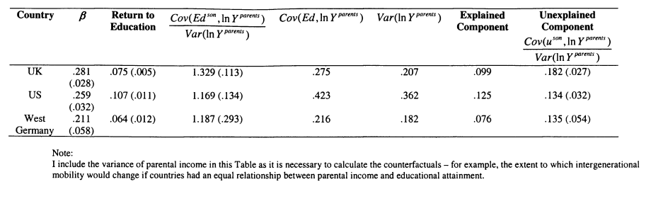
Appendix to Chapter 3

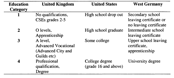
Chapter 4: Changes in Intergenerational Mobility in the UK and u s 22
4.1 Introduction
In Chapter 3 I have highlighted how comparisons of intergenerational mobility across countries can help us to understand more about the mechanisms which lead to limited mobility. Extending these comparisons to changes over time in mobility can help even more, as between country differences are fixed and we can begin to speculate about how policy and institutional changes affect mobility. In this chapter I compare changes in intergenerational earnings mobility for the US and the UK. Once again, methodological considerations are vital, and some time is spent in considering the robustness of the results given the limited nature of the data available.
In the UK I compare the extent of mobility for sons in the 1970 cohort (used in Chapter 3) with mobility in an earlier cohort of those bom in 1958.1 find strong evidence of a fall in mobility for the UK. I compare this with changes in mobility for the US using the PSID over similar cohorts of young men. Owing to the small samples available in the PSID I approach this question in several ways and find no significant change over the period of interest, although there is some evidence of an up-tum in intergenerational persistence for the most recent cohort.
The case of the UK and US is particularly interesting as these countries have both experienced large rises in income inequality since the late 1970s (Gottschalk and Smeeding, 1997). Cross country comparisons tend to suggest strong income persistence in the UK and US compared with more mobility in the Nordic countries. This leads us to imagine a positive link between cross sectional inequality and income persistence. This hypothesis has often been alluded to in the literature, but has not been formalised or conclusively explored (e.g. Hout, 2003, 2004). In particular, there is no evidence concerning the relationship between changing inequality and mobility.
Dickens and Ellwood (2003) show how wage inequality has combined with changes in work and demographics to lead to increases in relative child poverty in the two countries over the same period. Increasing relative poverty may
22 The work on the UK in this Chapter builds upon the research reported in Blanden, Goodman, Gregg and Machin (2004).
be one route by which increases in inequality lead to changes in mobility. If more relative poverty leads to more families being affected by credit constraints, or severer constraints for some families, then we might expect that increased inequality will lead to a reduction in mobility.
Some of the rise in income inequality since the late 1970s has been a consequence of increased returns to education (as illustrated by Machin, 1999 for the UK and Katz and Autor, 1999, for the US). Solon’s (2004) model of changes in mobility is very clear on the effect of rising returns to education (as, indeed, is the decomposition shown in the previous chapter). Expected returns will influence parental investment. If parents anticipate higher returns to human capital investment they will make more investments if they can afford to, leading to a larger gap between the human capital of those from richer and poorer backgrounds. Higher realised returns will lead to a stronger relationship between human capital investments and children’s income, generating another positive link between rising inequality and increasing intergenerational persistence.
Solon’s model also has several other predictions. The first is that the increased heritability of endowments across generations will lead to increased income persistence. As discussed in Chapter 2, endowments include everything that is transmitted between generations without investment decisions being made. The inherited component of immobility is inevitably somewhat of a black box. The advantage of considering changes in intergenerational mobility in the same countries is that, hopefully, some of the factors in this black box will remain constant over time.
The other mechanisms mentioned by Solon are more explicitly policy relevant, in that they consider the balance between public and private investment in children’s human capital. Solon shows that parental investments (and, consequently, intergenerational persistence) will increase with the productivity of parental human capital investment, and will fall with the progressivity of government investment. Conceptually, it is somewhat difficult to separate these two components. We can imagine that parental investment will be more productive when the investment provided by the government is low, investments in teaching a child to read will be very productive whereas additional cello lessons may be less so. It is harder to imagine what else may influence the efficiency of parental investments. Nonetheless, it is clear that increased government investment is likely to lessen the difference between the human capital of those from richer and poorer families and thereby increase intergenerational mobility.
Solon’s emphasis on government investments illustrates the possible importance of changes in education policy in the two countries. As the direct costs and foregone eamings associated with education increase substantially at the end of the compulsory stage it is common for credit constraints to be discussed primarily in the context of further and higher education. In Chapter 5 I focus on how changes in education policy have influenced the relationship between parental income and educational attainment in the UK, so I provide only a short summary for both countries here.
The overall story is that there has been a large expansion in postcompulsory education in the UK since the 1970s, at both the further and higher education level. This has been coupled with a cut-back in means-tested support for university students. Both of these points shall be discussed in considerable detail in Chapter 5.
In the US, the increase in enrolment rates has been more muted. Card and Lemieux (2000) show an analysis of enrolment by age, sex and year and demonstrate that while college enrolment rates rose slowly for women from the 1970 onwards enrolment for men dipped somewhat in the 1970s before rebounding. Enrolment rates for men at age 19 increased from around 40 percent in 1980 to 55 percent in 1996. The direct costs of attending university are substantially higher than in the UK, and there have been much less dramatic changes in the educational attainments of young people. The assistance available for young people in the US takes several forms, including means-tested (Pell) grants, subsidised loans and state-subsidised colleges and universities. Over the 1980s and 1990s fiscal stringency meant that fees at public colleges rose and loan limits were frozen. For more on the financing of higher education in the US, see Kane (1999) and Dynarski (2004).
In this chapter I focus on students who would have attended university between the 1970s and late 1980s. In the UK, the younger students would have been at the beginning of the large expansion of higher education, while later cohorts in the US would have been feeling the start of cut-backs in Government subsides.
In the next section I review the previous literature on changes in intergenerational mobility in the US, UK and other countries. In section 4.3 I discuss the data, while in Section 4.4 I consider the estimation approaches taken. Sections 4.5 and 4.6 provide a review of the results, with an emphasis on the robustness of my findings. Section 4.7 discusses the implications of this chapter, and Section 4.8 concludes.
4.2 Current Evidence
Measuring changes in intergenerational mobility over time has become a growing area of research, especially for the US. Several papers have now addressed changes in intergenerational mobility in the US, although none seem to satisfactorily address the issue in a way that is comparable with the data we have available for the UK. In addition, the studies have produced mixed evidence, so there is value in considering the question once more.
The main difficulty in considering changes in mobility in the US is that the main dataset available, the PSED, yields rather small sample sizes. This has been illustrated clearly in Chapter 3, and the problem worsens when the objective is to measure persistence across several time periods. Corcoran (2001), Fertig (2002) and Mayer and Lopoo (forthcoming) (known as henceforth as M-L) split the available data by cohort, choosing one value to represent the earnings (or family income in the M-L case) of the individual (Corcoran and Fertig both use an average measure, but there is still just one observation per individual).
Corcoran uses those bom between 1953 and 1968 and splits the data at 1960 to create two samples to compare. Parental income is observed over as many years as possible between age 8 and 17 and son’s earnings are the average taken over ages 25 to 27. Fertig’s method is less clear as the five cohorts she uses are based on the years in which parental income is observed, but not the child’s age specifically. M-L measures parental income when the child is aged 19-25 while adult family income is observed at age 30 for cohorts bom from 1949 through 1965. The number of individuals observed for each birth cohort at age 30 is very small. This difficulty is partly overcome by comparing rolling cohorts which include three birth-years of observations. All three of these studies find that the intergenerational elasticities have decreased over time in the US, but the changes observed are often on the margins of statistical significance.
Levine and Mazumder (2002) supplement these studies by using the National Longitudinal Surveys (NLS) and the General Social Survey (GSS) in addition to the PSID to explore US trends. They also find evidence of an increase in mobility using the PSID but a fall in mobility is found in the NLS surveys. Evidence from the GSS does not paint a consistent story. Unfortunately, both the GSS and NLS have their own problems as sources of data for intergenerational mobility. In the GSS there is no parental income measure, so income must be imputed either on the basis of the child’s five category retrospective report of relative income, or on the basis of father’s occupation and industry. There is also a problem with the parental income data in the NLS: in the first survey this is reported by sons and in the second by parents. This means that additional measurement error alone may be responsible for the lower estimates observed for the first survey.
The purpose of a new paper by Lee and Solon (2004) is to obtain estimates on changes in intergenerational mobility over time for the US which use the PSID but are based on much larger samples and are therefore more reliable. Lee and Solon use all the earnings observations available for children aged 25 and over in the PSID between 1978 and 2000 and regress these on parental earnings averaged over ages 15 to 17. This method means that the number of observations used and the ages at which earnings observations are taken is related to the birth cohort. The intergenerational coefficient obtained for each year of earnings data will result from time, age and cohort effects. For my purposes cohort effects are the main interest as we wish to compare the life chances of children bom at different points in time. The authors admit that cohort effects can only be separately identified if the age-eamings profiles of the different cohorts are identical over time, a nontrivial restriction. The conclusion of Lee and Solon’s work is that intergenerational mobility is constant across time for the US.
This review has illustrated that there is no ideal solution for measuring changes in intergenerational mobility in the US; all the available data has limitations. However, the PSID appears to be the most suitable data available. In this chapter, I focus on methods similar to both Corcoran and M-L to discuss changes over time in ways which are comparable with the data available for the UK. However, the clear limitations with these approaches mean that I take particular care to focus on the robustness of my results.
For the UK, research on changes over time is much more limited and the research presented here is the first to consider changes in intergenerational income mobility. Goldthorpe and Mills (2004) and Ermisch and Francesconi (2004) have measured changes in social mobility using occupation based social class measures and indices. Both studies find that the intergenerational connection between occupational status has declined over time. The interpretation of these results is complicated by changes in the underlying structure of social class and occupation over time. While the meaning of income may also change somewhat due to changes in the services provided by the non-market sector, my preferred measures of mobility use income, not least because income provides more variation and is easy to break down into equal-sized groups for ranking.
As discussed in Chapter 2, there are a number of papers which study changes in intergenerational mobility in other countries. The evidence from these suggests either no change or a decrease in intergenerational persistence over time. Taken as a whole, the current literature tends to point towards an increase in mobility. In this context, the evidence I find for a sharp fall in mobility in the UK is particularly striking, and leads us to question which factors have led to such a unique result for the UK, compared with other countries.
4.3 Data
UK Data
The two cohorts used in the UK comparison are the National Child Development Survey (NCDS) and the British Cohort Study (BCS). The BCS is used in the cross-country comparison in Chapter 3, and, as discussed there, includes all individuals bom in a single week in April 1970. The National Child Development Survey features the cohort bom in a week in March 1958, twelve years earlier. While the BCS has information on the cohort members at age 5, 10, 16 and 30, the NCDS has data collected at ages 7, 11, 16, 33, and 42. The important sweeps of data for my purposes are the age 16 sweep for both cohorts and the age 30 sweep for the BCS and age 33 sweep in the NCDS. At age 16, income information is provided by parents in both cohorts, while in the early 30s, information is obtained on earnings.
The parental income data is not provided in an ideal form in either cohort. The information on NCDS income is presented by source “father’s earnings”, “mother’s earnings” and “other income”. In each case parents are asked to provide information by selecting the band into which their net weekly or monthly income from each source falls. There is some ambiguity in terms of what missing reports for each component mean: does it mean that families have no income from this source or simply that the information is missing? If it is the case that a component is missing then there is an argument for dropping the observation. This issue is considered in some detail in a data note by Micklewright (1986) and I have followed his advice in excluding families where a parent’s earnings are missing but they are reported to be working in another part of the questionnaire. The BCS parental income data is not reported by component. Instead, parents are asked to indicate which band (from 11) their gross total weekly income falls into.
In order to use banded data as an explanatory variable in the usual intergenerational model I must convert it into a continuous form. For the NCDS I assign each component a single value which is the midpoint for this component for similar families in this band in the Family Expenditure Survey (FES) in 1974. Family income is generated by summing these variables. Combining information on three components means that the final income distribution has 77 different values. For the BCS, where there is only one banded variable, I use maximum likelihood estimation to model a Singh-Maddala distribution for the data, as in Chapter 3. In principle, it should also be possible to estimate the distribution based on the 77 unique categories in the NCDS, but the fact that the upper and lower bounds for the categories are not exclusive means that this is computationally impractical.
The methods of data collection indicate some clear problems with the comparability of the parental income data across the cohorts. First, there are clearly many more unique values possible for the NCDS than the BCS. Second,the NCDS income components are reported as net of tax while the BCS asks for gross income. To account for this, I refer across to the FES data for the appropriate year (in this case 1986) where incomes are reported both net and gross. I can then calculate the proportion paid in tax by families in each band. I subtract the median of this from the expected value obtained in the SinghMaddala distribution23. The final difficulty is that the NCDS income question clearly asks parents to include child benefit, whereas the BCS data asks that it be excluded. I therefore impute a value for child benefit based on the number of children in the household (and lone parent status for the BCS). My initial estimates use data where this amount is added to the BCS income, but I also experiment with subtracting it from the NCDS instead.24
There is one final concern with the parental income data, which relates to the NCDS only. In 1974, when the age 16 data was being collected for this cohort, Britain was in the midst of a three-day working week due to a power shortage brought about by unrest in the coal industry. The worry is that parents would report their incomes from a three-day week rather than their usual incomes. Grawe (2004c) considers this difficulty by comparing reported father’s earnings across the period when the three-day week was in effect with information gathered after it had ended. The study seems to find convincingly that few income reports have additional measurement error due to the exceptional circumstances and Grawe states that his best estimate of the fraction of misreports is zero.
Compared to these difficulties, the cohort members’ earnings data available for the two cohorts are more straightforward to use. For both cohorts individuals are asked to provide information on their gross and net pay and state the period which each covered. I use gross pay in my analysis to be comparable with the information available in the US data, and convert this to monthly figures. Unfortunately, there appear to be a number of cases in which the pay period has been incorrectly coded; consequently this data has been carefully cleaned. Inevitably, an element of judgment is in play, but the cases which need attention are generally obvious due to either extremely high or low weekly earnings or
23 The proportion subtracted in tax is zero for the first two income bands (up to £100 a week in 1986 prices) and rises up to 26% in the top income band (those with incomes of £500 or more). 24 Child benefit rates for 1974 and 1986 were obtained from the Institute for Fiscal Studies web site http://www.ifs.org.uk/taxsystem/contentsben.shtml.
hourly wages, or great inconsistency between the net and gross weekly earnings (different pay periods are asked for each measure). Both sets of earnings data used here have been cleaned independently by colleagues at the Institute for Fiscal Studies and the changes made generally match up well between the two versions, (for example, the correlation between the two versions of the BCS earnings data is .82). As discussed in Chapter 3, a limitation of the BCS data is that information on self-employment income is poor, this is also a problem in the NCDS. Consequently, the self-employed are dropped from both datasets, as are those not in employment at the time of the survey.
In summary, the comparisons made over time for the UK rely on a comparing the relationship between parental income at age 16 and individual earnings at age 33 for a cohort bom in 1958, with the relationship between parental income at age 16 and earnings at age 30 for a cohort bom in 1970. The comparison is necessarily based on two snap-shot measures, and this limitation must be borne in mind when we extrapolate to draw conclusions about the trends in intergenerational mobility in the UK.
The discussion in the preceding chapters has made the point, time and again, that measurement error in the parental income measure can lead to serious biases in the estimation of intergenerational mobility. The fact that the UK estimates rely on single week (not even single year) measures of parental income is therefore of some concern. The instrumental variables solutions proposed in Chapter 2 are unsuitable here, experimentation has shown that using education and social class as instrumental variables in the cross-cohort context is dubious. Sargan tests indicate that the extent of upward bias introduced by these variables varies substantially across the cohorts and that estimates seem to be very sensitive to the choice of instruments. The difficulty posed by measurement error in the explanatory variables is therefore of great concern, the most important dimension of this is the extent to which the extent of measurement error varies across the cohorts. The robustness of the results to measurement error will be considered in detail.
A further concern about these data is the extent of attrition and item nonresponse in the two cohorts, the combination of these two data problems means that only one fifth of the original cohorts can be used in the intergenerational analysis. Once again, the concern is that these difficulties may lead to different biases in the two datasets, meaning that the results are not legitimately comparable. This issue is addressed in some detail in the appendix; however, I flag up the key implications of my analysis in the results section.
US Data
The PSID data used to estimate changes in intergenerational mobility over time in the US has been discussed in some detail in Chapter 3. To recap, this survey follows a national sample of households from 1968 to the present, following all members as they split from sample households to form new households. In many ways this data is highly suitable for considering the trend in intergenerational mobility as it is collected every year and available for all birth cohorts. The difficulty is that the numbers of observations available for a particular birth cohort are limited, as has already been discussed.
I measure parental income in the same way as in Chapter 3. Parental income is taken as the total family money measure less the earnings of members other than the “head” and “wife”. In the analysis which is comparable with the UK, I average parental income over ages 14 to 18. Sons are matched to parents on the basis of the head of the household in which the son lives at age 16 (provided he is classified as a “child” in the household); this is in contrast with the approach of M-L, who use the parental identifier file to match children on parents, as commented upon further below. These two decisions are taken to ensure comparability with the information in the UK data where family income is the income of the “parents” who live with the child at age 16.
The sons’ earnings used as the earnings for the year the son turns 30, obtained when he is 31. For the sons who turn 31 in 2000 or 1998 (the years when there was no survey) data for the following years is used. Those who report themselves to be self-employed at the time of the survey are excluded.
The PSID is composed of two sub-samples: the nationally representative Survey Research Centre sample (SRC), and the Survey of Economic Opportunity (SEO) which focuses on the disadvantaged. Lee and Solon (2004) and Fertig (2002) discard the SEO (as do I in Chapter 3), while M-L include the additional observations and use the weights provided to account for the over-sample. The benefit of this is that the effective sample size increases. I show results which both include and exclude the SEO in order to discover whether this decision has important implications.
I take two broad approaches to the data. First, I split the data by birth cohort into three exclusive samples, those bom 1954-1957, 1958-1962 and 1963- 1970; this is similar to the approach chosen by Corcoran. Second, I use the rolling birth cohort approach use by M-L. I begin the rolling cohort analysis by replicating M-L’s analysis as far as possible for cohorts bom from 1949 to 1965.1 then modify this approach to be as comparable as possible to the UK cohorts and consider sons bom up to 1970.
Replication of M-L’s estimates is important. The criticisms of the smallsample approach to measuring changes in intergenerational mobility are in part due to the fear that the results found are due to specific decisions concerning sample selections and variable use. If results from this approach are to be taken seriously, it is necessary to show they are robust to different approaches. In particular, M-L use parental income measured between ages 19 and 25 and use family income, rather than earnings, as the dependent variable. It is important to know what impact these decisions have on the results. In addition, it is necessary to show how results for later cohorts (not considered in the M-L analysis) are related to those for earlier groups. The main finding of the M-L paper is that the intergenerational elasticity declined for sons bom between 1953 and 1965. The two questions I address are: is this trend still present when data is used which is more comparable to what I have in the UK, and does it continue for cohorts bom from 1965 to 1970?
4.4 Estimation Approaches
As in Chapter 3, I focus on two measures of intergenerational persistence; the intergenerational elasticity ( Pcj) and the intergenerational partial correlation ( rcj), the parameters and variable are subscripted by cohort c in country j as these are the two dimensions which are varied in this analysis.
As before, /? is obtained from a regression of son’s earnings on parental income, as in equation (4.1).


The partial correlation is obtained by adjusting /3 by the ratio of the parents to child’s standard deviations of income/earnings.
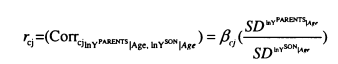

As in Chapter 3, the virtue of the correlation measure is that it will be invariant to differences between the variances of sons’ earnings and parental incomes. This will adjust for changes in inequality between the two generations, and the fact that the change in inequality between parents and children may vary by birth cohort as aggregate inequality increases in both countries.
4.5 Changes in Intergenerational Mobility in the UK
Table 4.1 shows descriptive statistics for the data used to investigate intergenerational mobility in the UK. This table confirms that we are considering two cohorts facing an era of increasing inequality. There is more earnings inequality for sons in the BCS than the NCDS, and parental incomes are more unequal among the second cohort than the first25.
Table 4.3 reports the first estimates of changes in intergenerational mobility in the UK. For sons bom in 1958 the elasticity of own earnings with respect to parental income was .205; for sons bom in 1970 the elasticity was .291. This is a clear and statistically significant growth in the relationship between economic status across generations. For the correlation estimates, the fall in mobility is even more pronounced. The correlation for the 1958 cohort is .166 compared with .286 for the 1970 cohort. The correlation is lower than the elasticity for the 1958 cohort because of the particularly strong growth in
25 The parental incomes reported here for the BCS are different from those reported in Table 3.2 as parental incomes have been adjusted for tax and child benefit as explained in the data section. The sample is also larger as in Chapter 3 I imposed the restriction that income data should be available at ages 10 and 16.
inequality between parental income and son’s earnings (in other words, s d 58’”’!°’W > y This is no surprise when we remember that parental income was collected in 1974 whereas sons’ earnings were measured in 199326.
Initial results suggest that the intergenerational mobility of sons has decreased between the 1958 and 1970 cohorts in the UK. However, given the complications and difficulties noted in the data section, it is important to give the robustness of this result thorough consideration. I now produce a number of pieces of evidence in support of my initial result.
As explained in the data section, the form of the two datasets is far from ideal, and some adjustments have been made to get the data in the form shown in Table 4.1. First, I experiment with the adjustment for child benefit. To recap, the NCDS data comes in bands for three components of net income, an expected income is assumed for each band and component and the resulting values are added. In the BCS, gross income (less child benefit) is measured on an 11 category scale and appropriate expected values for each band are computed by fitting a Singh-Maddala distribution.
In order to make the BCS data more comparable with what is available in the NCDS, a proportion is removed for tax and imputed child benefit is added. It would be unreasonable to completely ignore these difficulties. An alternative would be to calculate the child benefit which is received by the NCDS families and subtract this from the NCDS income instead. When this is done, the change in the elasticities falls slightly to .063 (.033) compared to .085 (.036) moving it on to the margins of statistical significance. However, the change in the correlations remains strongly significant at .110 (.033).
Ultimately, the refutation of the results presented in Table 4.2 depends upon the NCDS estimates suffering from greater downward bias than the BCS estimates. As discussed in previous chapters, Haider and Solon (2004) have shown that downward bias can come from measuring sons’ earnings at an early
26 Differences between the results for the BCS in Table 4.2 and those in Table 3.3 are due to differences in the measure of parental income, as described above. The difference is larger for the unadjusted results (betas) because accounting for tax and child benefit equalise parental income, leading to higher estimates of beta.
age. However, since the NCDS data is observed at 33 compared with age 30 in the BCS, this is unlikely to be responsible for the differences between the cohorts Any differential downward bias is likely, therefore, to result from poorer measurement of parental income data in the NCDS.
Table 4.3 shows a calibration exercise on how much larger the measurement error would be required to be in the NCDS for us to conclude there is no statistically significant rise in the partial correlation for sons across the cohorts, for various assumptions on measurement error in the BCS. For example, the first row of the Table shows that if we assume complete accuracy in the BCS one would require measurement error in the NCDS to be 26 percent for sons. As I relax the assumptions on the accuracy of the BCS data, it is clear that the measurement error required in the NCDS to get rid of the rise also increases and is often substantial. For example, if measurement error in the BCS is as high as Mazumder’s (2000) recent paper suggests, the NCDS measurement error would need to be 73 percent for the rise we observe to be rendered statistically insignificant. Table 4.3 shows under various assumptions that there would need to be substantially higher measurement error in the NCDS data to eliminate the pattern of rising intergenerational immobility across the two cohorts.
Transitory income variations are the main form of measurement error in parental earnings or income mentioned in the literature. The problem is especially acute here as parental income is just a single weekly measure. In order to get a handle on the effect this may have on my estimates, I have investigated changes in the permanent versus transitory component of labour income in a large British data source, the New Earnings Survey panel. The New Earnings Survey is a one percent employer reported database covering all British employees carried out in April of each year. It contains very accurate wages data from employer records and enables one to follow people through time. This data can be used to work out the permanent and transitory components of earnings and compare them with the NCDS and BCS data.27
27 Dickens (2000) undertakes a detailed study of how much of the rise in earnings inequality seen in Britain is due to a rise in the permanent versus the transitory components of earnings. He finds about half of the rise in the variance of hourly earnings between 1975 and 1995 to be permanent, and half transitory.
If the relative importance of the transitory component of income has decreased over time, then this provides some independent evidence from another data source for the possibility of higher attenuation bias in the NCDS. It seems that the data is partly in line with this. Estimating a fixed effect earnings equation over five years of data for a cohort equivalent to the BCS fathers shows that transitory fluctuations in income account for 21 percent of the total variance. A comparable figure for NCDS fathers is slightly higher at 32 percent. However the last row of Table 4.3 shows the variance contribution of transitory income would need to be higher than this, at 44 percent, to result in no statistically significant fall in mobility. In summary then, Table 4.3 shows that measurement error in the NCDS would need to be quite substantial to even reduce the observed rise to statistically insignificant levels, let alone to account for it entirely.
In the appendix I consider the implications of attrition and non-response for these results. While it is very difficult to be entirely confident about how results will be driven by selections into the sample on unobservable characteristics, the evidence available suggests that the finding that intergenerational mobility has declined reflects a real change rather than being driven by data weaknesses. Therefore, all the evidence presented so far encourages us to believe that there has been a genuine rise in the link between the incomes of parents and their sons in the UK. The next step is to find out whether similar trends are observed in the US.
4.6 Changes in Intergenerational Mobility in the US
The PSID data is much more flexible than the data used for the UK. I exploit this flexibility, and take a number of approaches to measuring changes in intergenerational mobility.
Three Cohort Analysis
Table 4.4 shows descriptive statistics for three cohorts: those bom 1954-1957, 1958-1962 and 1963-1970. After 1996 the sample was reduced quite substantially (dropping many of the SEO families) which is why I include more birth years in the final cohort than in the first two. One of the decisions which must be made when using the PSID is whether to include the SEO sample and weight the data. I have therefore shown the descriptive statistics for both the weighted and unweighted data, where the unweighted data excludes the SEO. The unweighted data generally seems to have very slightly higher means. This is likely to be because the weights take account of differential attrition as well as initial sample differences. In general, the patterns for the weighted and unweighted data are very similar. There is clear evidence of growth in both parental income and sons’ earnings across the three cohorts. Inequality in parental income appears to fall between the first and second cohorts and then rise between the second and third cohorts. This makes sense, as parental incomes for the cohorts were obtained in the early 1970s, the mid to late 1970s and the late 1970s and onwards.
Table 4.5 uses these three cohorts to produce my first estimates of the changes in intergenerational mobility in the US. Once again, I present weighted estimates in the upper panel and unweighted estimates in the lower panel. What is immediately clear is that none of the changes in elasticities or correlations are statistically significant. Putting aside the issue of significance, the point estimates suggest an overall rise in intergenerational persistence between these three cohorts; the opposite trend to the one reported by most of the current papers on intergenerational mobility using the PSID. This trend is most apparent between the second and third cohorts. These more recent cohorts are not generally used in current studies, so there is a possibility that by extending the samples I am picking up a trend which has not been examined before. Reassuringly, results do not differ substantially between the panels, for either the level or the change. This adds to my confidence about the results reported in Chapter 3, which are based on excluding the over-sample, this decision will not have made much difference.
Owing to the small samples used, Table 4.6 does not allow strong conclusions to be drawn about changes in intergenerational mobility. It is also clear that the insignificant rise which is observed could be a consequence of the way that the data is split into periods; the effect of moving one birth year between cohorts is unclear. Consequently the remainder of the analysis compares results based on rolling cohorts, which show how robust the results are to changing the definitions of the cohorts.
Rolling Cohort Analysis
The starting point for this analysis is Mayer and Lopoo’s forthcoming paper, (ML). This paper explores the relationship between family incomes across generations, my approach is to move in a step-by-step way from M-L’s analysis of family income mobility for cohorts from 1949 to 1965 to my UK-comparable analysis of sons’ earnings mobility for cohorts from 1954 to 1970. The first step is to replicate M-L’s analysis. I have not been able to be completely precise in this replication and Table 4.6 shows how my sample sizes differ from those reported in M-L. In every case, my samples are slightly larger than those used by Mayer and Lopoo, by around 5 percent. It appears that the authors are placing some restrictions on the data which are not obvious by their descriptions in the text.
Figure 4.1 and Table 4.7 show how the results from my replication differ from those in M-L’s paper. In the initial cohorts the elasticities I present are quite a lot higher than M-L’s results, however from 1953-1956 to 1960-1963 the results are extremely similar. Figure 4.3 demonstrates clearly that my replication shows the same overall pattern as the M-L results, particularly with regard to the fall in the elasticity from 1953 onwards. Mayer and Lopoo do not report the correlation coefficients in their paper. However I show the appropriate correlation coefficients for my replication. These suggest a flatter trend in intergenerational persistence than the elasticities. This is because the difference in inequalities across generations reduces for later time periods, as parental incomes begin to be affected by rising inequality. For the final cohort parental incomes are observed during the 1980s. Changes in inequality may, therefore, lead to an over-statement of the fall in intergenerational mobility over this period. Consequently I report both correlations and elasticities from now on.
The first step to move from M-L’s approach to one more comparable with my UK analysis, is to use earnings rather than family income as the dependent variable. The connection between family incomes across generations is undoubtedly very interesting, and is considered in great detail in Chapter 6. However, this compounds many influences, including the age of family formation, wives’ labour market participation and child-bearing decisions. The impacts of these in the US are discussed in more detail in Mayer and Lopoo (2004). In this chapter I wish to focus on sons’ individual earnings. Figure 4.4 shows the results from my replication of the M-L approach for both family income and earnings as dependent variables. Again, the trends are similar, but with earnings mobility somewhat flatter over time than family income mobility. In fact, when we look at the partial correlation for earnings, the trend appears to be almost flat across the whole time period.
So far my results indicate that the evidence for an increase in intergenerational mobility does not seem to be as strong as an initial glance at the literature may suggest. I now make a few final modifications to ensure that the analysis is as comparable as possible with what I have for the UK. The parental income data used in the M-L replication is obtained from parents at age 19-25, this seems rather late. The one advantage of using this data is that it enables the use of older cohorts who would have been teenagers before 1968 when the survey started. However it seems more natural to want to know about the connection between sons’ earnings and their parental income in the teenage years, when investments are actually being made. Also, the information on British parental income is taken at age 16; I therefore use parental income data at age 14-18. In addition, I change the way that parents and children are matched. Mayer and Lopoo use information from the parental identification file, instead, I use information about who the child is living with at 16. Both of these changes mean the income measured is more likely to be relevant to the investments made in the child.
In Table 4.8 and Figures 4.3 and 4.4 I show the difference that these modifications make, and provide results for later cohorts up to 1970. I show results for ft coefficients and partial correlations separately. In both cases I report three sets of estimates: the first is for my replication of the M-L approach (parental income measured from 19 to 25) with earnings as the dependent variable; the second shows the same sample but using parental income between ages 14 and 18; and the final results show estimates for cohorts up to 1970, using parental income from ages 14 to 18 and matching parents on the basis of who the child lived with at age 1628. It is clear that for the cohorts where the three estimates overlap, the different estimation methods have a limited impact; there
28 The other slight change is that M-L use 1995 weights, for my final estimates I use age 30 weights. This has very little impact on the estimates.
are certainly no differences which approach statistical significance. However, extending my preferred estimates into later cohorts shows a very sharp increase in the point estimates of the intergenerational elasticities and partial correlations.
The picture from point estimates of the /? coefficients is one of increasing mobility up until the 1957-1960 cohort, followed by a flat period and then a strong fall in mobility (rise in J3) for the 1964-1970 cohorts. For the partial correlation results the initial upward trend in mobility is less clear. However, the kick up in the estimate for the last cohorts is still very much in evidence; and it is also found when the Survey of Economic Opportunity is excluded from the sample and weights are not used . I have experimented with a variety of functional forms to capture these patterns in the data, but have been unable to find any statistically significant trends.
It is unfortunate that there are no datasets which could provide more sizable samples of data over this period. A strong finding of increasing mobility followed by a fall shortly afterwards would be extremely interesting and may make us wonder about the connection between intergenerational mobility and the business cycle, for example. However, given the sample sizes that are available the only solid conclusion I can draw is that there are no significant changes in the US over the period of the British data, nor going back to cohorts dating from 1949.
4.7 Discussion
To reiterate, the main story which has emerged from this chapter is one of falling intergenerational mobility in the UK. The picture for the US is of fairly stable intergenerational mobility but with a possible fall in mobility for the most recent cohorts.
As I discussed in the introduction to this chapter, both of these countries experienced a sharp increase in cross-sectional household inequality over the period under consideration. One of the motivations behind this chapter is to assess
29 A possible explanation for the very recent change in the estimates o f would be the reduction in the sample from 1997 onward. I have repeated the analysis in Table 4.10 on only those individuals who are still in the sample from 1997, and there is no evidence to suggest that this explanation is correct.
if the rise in cross-sectional inequality is matched by an increase in intergenerational inequality. The evidence for the US suggests that it is not. At least, if there is a close link between inequality and intergenerational mobility, then there must be countervailing factors in the US which have worked in the opposite direction, at least for cohorts bom up to the late 1960s. One explanation is that relative child poverty is more important than inequality per se. Dickens and Ellwood (2003) show that increases in child poverty were much stronger in the UK than the US as inequality rose from the late 1970s onwards.
An alternative candidate explanation for the changes observed is the role of education, both through returns and through the relationship between parental income and education. In the next chapter I provide a full consideration of the relationship between changes in intergenerational mobility and educational attainment in the UK. I show that changes in education participation have helped to increase intergenerational mobility in the UK, with educational changes (driven by an increase in the relationship between parental income and education) explaining at least 30 percent of the overall change.
The evidence for the US suggests that the rise in returns to education did not have the correct timing to account for the rise in persistence observed at the end of my data, while there is little evidence on recent changes in the education – parental income relationship.
Angrist, Chemzhukov and Femandez-Val (2004) show a rise in the schooling coefficient in an earnings regression from .07 in the 1980 census to .11 in the 1990 census. The return to education is then constant between 1990 and 2000. The implication, therefore, is that increases in the returns to education in the US could not explain an increase in intergenerational persistence among very recent cohorts.
Evidence on changes in the relationship between parental income and educational attainment in the US suggests that parental income has had an increased impact on children’s attainment. By comparing the High School and Beyond Survey of the class of 1982 with the National Educational Longitudinal Survey of 1988 Kane (1999, pl26) finds that increases in participation at four year college over the 1980s were disproportionately focused on young people with higher household incomes. Similarly Manski (1992) finds an increase in the relationship between education and parental income in Current Population Survey from 1970 to 1988. More recent evidence on the relationship between education and parental income is limited.
The findings in the literature on returns to education and the educationparental income relationship would encourage us to expect a rise in intergenerational income persistence in the US throughout the data, but as I have noted, this is only observed in the very last periods of data, if at all. It is hard to think of an explanation for a dramatic increase in persistence in recent periods; there is no obvious policy change which would produce them. In order to get some sense of the forces operating I have repeated the decomposition from the previous chapter on each period. The evidence from this suggests that the large rises in the elasticity are largely unexplained by education.
As noted above, education does a better job at explaining the change in intergenerational mobility in the UK, explaining 30 percent of the change observed, and this will be returned to in the next chapter. However, a natural question is to ask what explains the remaining 70 percent of the increase in persistence. These explanations could also help to shed some light on why intergenerational persistence does not appear to increase in the US.
One initial candidate is the composition of families. We know that larger families tend to have more income, and also that larger families tend to have poorer outcomes per child (see Becker and Lewis, 1973). So far, this has not been accounted for in any of the estimates. To investigate this I devise rough equivalence scales30 and repeat the intergenerational estimation using equivalised parental incomes. The results from this exercise show that the family size can explain a small part of the change. Using equivalised income the partial correlation rises by .081 (an increase which is still statistically significant) compared to .119 in the non-equivalised results. The smaller change is explained by the rise in the intergenerational correlation when equivalised income is used in the NCDS; this is generated by the strong negative relationship between the
30 The equivalence scales used are based on McClements’ (1977) methodology, but missing information on the ages of the cohort members’ brothers and sisters prevent these from being as precise as they might be. Equivalised income is obtained by using these scales to derive income per adult equivalent.
family size and earnings at age 33 in this cohort, which is not apparent in the BCS sample.
Another aspect of family composition which may have implications for estimates of intergenerational persistence is growing up with a single mother. This could help to explain the aggregate changes observed if either the proportion of children with lone-mothers or the impact of this for intergenerational estimates has changed,. The data does not reveal any evidence that this can explain the increase in persistence. For both cohorts, the partial correlation estimate is slightly larger (by about .01) when children growing up with no father in the household at age 16 are excluded. As the proportion of these children with no father in the household has risen slightly between the two cohorts, the difference in intergenerational persistence along this dimension would contribute towards a fall in intergenerational persistence rather than the rise which is observed.
The intergenerational literature rarely assesses the impact of structural economic changes for mobility. One example of this would be changes in regional inequalities. As shown in Jackman and Savouri (1999) and Gregg, Machin and Manning (2004) the regional disparity in unemployment and employment rates grew extremely fast between 1979 and 1986, and while gaps in unemployment rates have closed through the 1990s, regional inequality in male employment rates remained wide through to 1999. The impact of this on intergenerational mobility can be expressed in a similar way to the impact of education on intergenerational mobility.
Regional disparities mean that sons’ income is a function of the region he lives in, gc represents the extent of regional inequality.
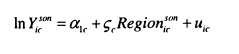

The region the son lives in as an adult can be thought of as a consequence of parental income. Here parental income represents two aspects of the influence of parental background on region of residence; the parents’ own region (the importance of which will depend on the migration rate, and the regional inequalities that effect parents), and the fact that those with high parental income tend to attain university education more move away from home (see Gregg, Machin and Manning, 2004, for more on the UK’s national graduate labour market). These relationships are captured by 07r , and (abstracting somewhat) more regional mobility for sons would lead to a reduction in mc between the cohorts.
![]()

The impact of regional differences on changes in intergenerational mobility therefore depends on the changes in regional inequalities and residential mobility between generations. To explain the fall in intergenerational mobility regional inequalities would need to have grown, while mobility declined among sons. Regional inequalities appear to have remained constant or fallen slightly between 1991 and 2000. The trend in the extent of regional mobility is less clear and appears to depend upon which data source is used; however there is no firm evidence pointing towards a fall in residential mobility across regions.
Although far from comprehensive, this discussion has served to illustrate how regional inequalities may impact upon intergenerational mobility, and demonstrate that in a simple model recent changes in regional inequality cannot explain the rise in intergenerational income persistence observed. A similar argument could be made in terms of changes in the industrial structure and would consider the returns to being in different industries and the influence of parental background on the sector of employment.
Esping-Andersen (2004) emphasises the importance of parent-child transmissions in early life for generating intergenerational inequalities. He particularly stresses the development of cognitive abilities (which are not as closely related to educational attainment as we might imagine) and the role of cultural capital and the family environment in generating these. He argues that the high quality childcare available in Nordic countries reduces the relationship between cognitive functioning and parental background that leads to intergenerational income persistence. The argument emphasising the importance of the early years in encouraging mobility is becoming increasingly common in the policy debate in the UK (see Alakeson, 2005).
For the mechanisms discussed by Esping-Andersen to explain the rise in persistence there would need to be either an increase in the association between family background and cognitive skills, or a rise in the return to cognitive skills in the labour market. The importance of these mechanisms are explored to a limited extent in Blanden et al (2004) where it is found that adding early test scores (proxies for cognitive skills) to the intergenerational model is unable to explain the change in mobility. Evidence on the role of other traits which are generated within the family and rewarded in the labour market is currently more limited, although an analysis of the role of non-cognitive traits in explaining intergenerational persistence is on the agenda for future research.
4.8 Conclusion
Comparisons of the 1958 and 1970 cohorts of sons in the UK indicate a large change in intergenerational mobility, such that the earnings of sons in the second cohort are much more closely linked to parental income than is the case for those bom twelve years earlier. This occurred over a period when income inequality was increasing for both parents and children.
Despite the growing number of papers which have examined the change in intergenerational mobility over time in the US, my findings indicate that the small sample sizes available for the US mean that the data is not well suited to measuring changes in mobility. The conclusion of much of the literature to date (Lee and Solon, 2004, excepted) appears to be that mobility in the US has increased in recent years. However, this conclusion appears to be fragile to changes in the dependent variable or to using the correlation rather than the elasticity as the measure of association. In addition, adding data for cohorts up to 1970 indicates that intergenerational persistence has rebounded in recent years, albeit not to a statistically significant extent. The overall conclusion must be that there has been no change in intergenerational mobility which is large enough to detect in the PSID.
It is natural to seek an explanation for the differences in the trends between the UK and US. Aside from the data issues, why is it the case that changes in intergenerational mobility in the UK are so much more dramatic? I have discussed a number of possibilities. The direct connection between crosssectional inequality and mobility does not appear to be directly responsible for the rise in intergenerational persistence in the UK, as the rise in inequality in the early periods for the US was stronger (although child poverty increased more quickly in the UK). Changes in education policy are the next likely contender, and changes in education policy and participation rates were greater in the UK than in the US over this period. As we shall see in the following chapter, education does explain some of change in the UK. Nonetheless, this is only responsible for part of the difference between the trends in the two countries and while I have discussed some likely candidates, the rest remains unexplained.

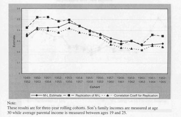

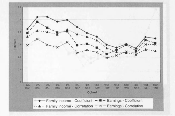
Mayer-Lopoo Approach

Replication and New Results

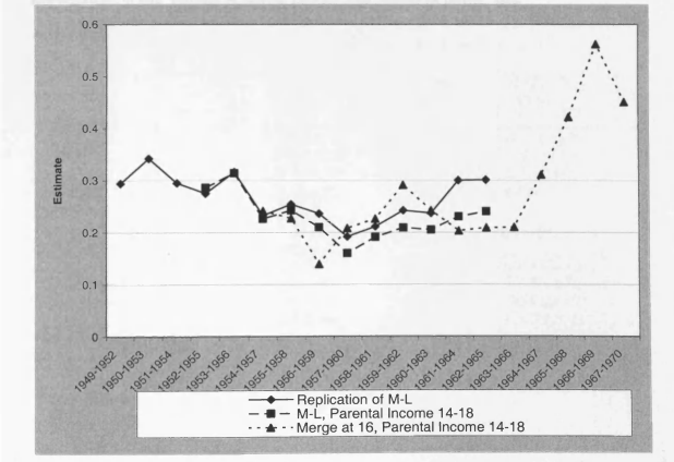
Replication and New Results

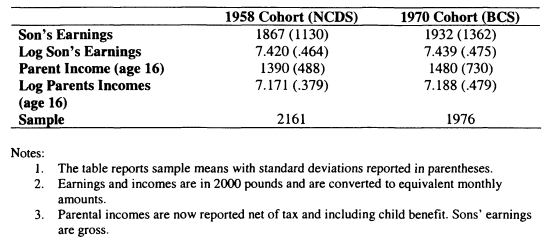

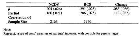

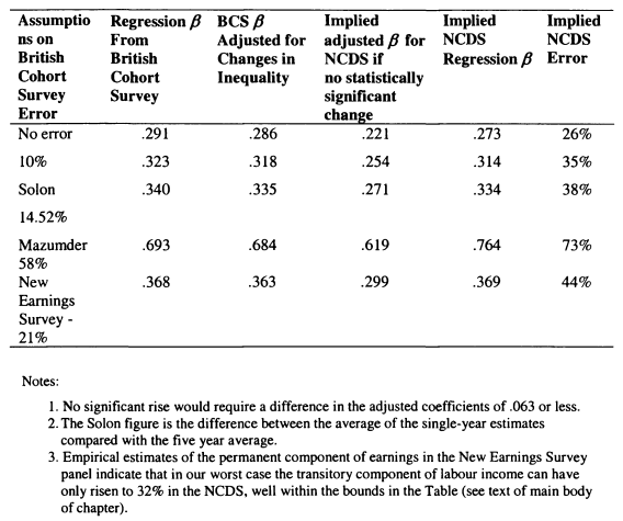

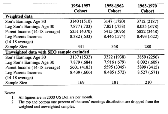

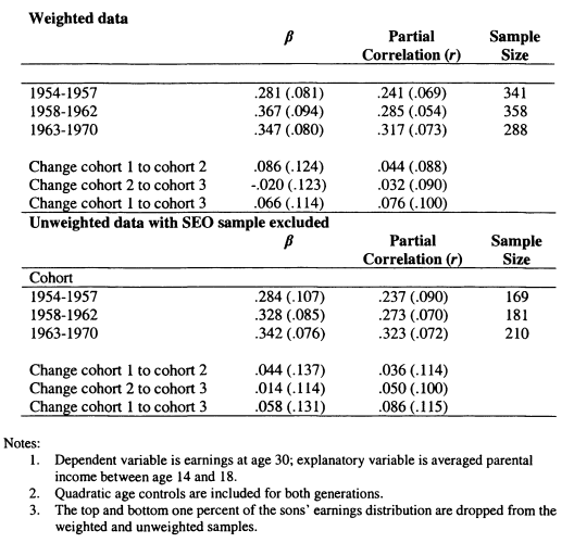
Changing Mobility in the US

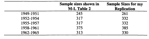

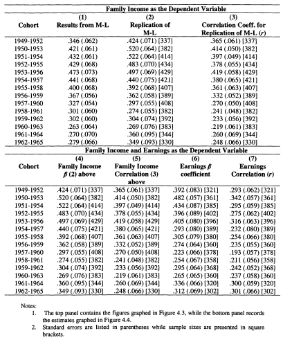

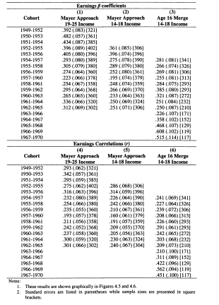
Chapter 5: The Role of Education in Generating Increased Intergenerational Income Persistence in the UK31
5.1 Introduction
There is a clear connection between the persistence of income inequality across generations and the unequal distribution of educational attainment. Young people from richer families have higher educational attainment than those from more deprived backgrounds, and this is one of the reasons that they go on to earn more. As a consequence, the equalization of educational attainment for children from different backgrounds is seen as an important policy tool to promote social mobility. This goal can be clearly seen in the rash of recent policies designed to improve the education prospects of those from poorer backgrounds in the UK (e.g. Excellence in Cities, Education Maintenance Allowance, see McNally, forthcoming, for details).
This chapter looks in detail at the relationship between parental income and educational attainment in the UK, demonstrating how this has changed over time. I then go on to investigate the extent to which the relationship between parental income and educational attainment can be regarded as causal, rather than simply reflecting inherited ability and other family characteristics which are correlated with income. This is important as without an understanding of what underlies educational inequality is it impossible to know how policy can be used to reduce inequalities and promote intergenerational mobility.
A strong motivation for the focus on changes over time is the evidence from Chapter 4 that intergenerational mobility for sons has fallen in the UK. I find that an increase in the relationship between educational attainment and parental income explains part of this trend. Specifically, I show results for educational inequality, measured as the gap in attainment between those from rich and poor backgrounds. Comparing the 1958 and 1970 cohorts once more, I find that educational inequality increased both in terms of staying on at school beyond age 16 and for access to higher education.
The relationship between parental income and education can also be considered for later cohorts, who are not yet old enough to have reliable earnings
31 The research described in this chapter has been carried out jointly with Stephen Machin and Paul Gregg. Published outputs are Blanden and Machin (2004), Blanden and Gregg (2004) and Blanden, Gregg and Machin (2005).
information (so cannot be used in a full intergenerational analysis). I extend my findings by incorporating information from the British Household Panel Survey (BHPS) on cohorts going through schooling in the 1990s. Evidence from these more recent cohorts (up to those bom in the late 1970s) is mixed, but the most telling measure (the relationship between higher education graduation and parental income) illustrates that there has been no reversal in the growth of educational inequality. This is potentially bad news for the mobility of these cohorts.
My analysis is presented for a period which saw sharp increases in educational attainment and post-compulsory participation in the UK. The key message is that despite the expansion of the number of students undertaking higher qualifications, the distribution of these opportunities was skewed towards students from higher income backgrounds. The importance of this evidence from a policy perspective cannot be overstated, especially as higher education policy is likely to be a key battleground in the 2005 general election campaign. Labour has nailed its colours to the mast by putting forward a 50 percent target for higher education participation (current participation is 1 in 3) and introducing top-up fees while the Conservative policy amounts to restricting the numbers in higher education and reducing the direct cost of study (Goodman and Kaplan, 2003). While the research reported here is unable to determine the precise impacts of these policies, it is clear that in the past (from the 1976 up until around 2000) expanding the number of places has not substantially improved access for those from poorer backgrounds.
My main findings on changes over time receive support from other studies. Galindo-Rueda and Vignoles (forthcoming) consider the interaction of income and ability in determining educational attainment. They find that while ability had a declining impact on educational attainment, the impact of parental background increased. Galindo-Rueda, Marcenaro-Gutierrez and Vignoles (2004) consider more recent changes in access to higher education. As information connecting participation with parental income is unavailable, two alternative approaches are used. By matching student postcode information with local income data, the authors find that the gap in participation between those from rich and poor neighbourhoods widened over the 1990s. In addition, they find that gaps in participation by social class widen from 1994/1995 onwards. The evidence on widening gaps in participation is further confirmed by very recent statistics from the Higher Education Funding Council (HEFCE) covering 1994-2000, who report that “most of the new places in HE have gone to those from already advantaged areas” (HEFCE 2005, p. 11)
My discussion of theoretical models in Chapter 2 showed intergenerational persistence to be a consequence of both the inheritance of endowments between generations and the investments made by parents in their children. I also noted how difficult it is to distinguish these two mechanisms in the data. The same argument applies to the relationship between parental income and educational attainment. Those with higher parental income have more education, but it is hard to discern whether this is because these children are brighter and more motivated, or if parental income actually makes a direct difference to the educational opportunities available to children. An understanding of this question is essential from a policy viewpoint as it will help us to appreciate if there will be a direct impact of policies to reduce child poverty on the education of children, or if alternative interventions are necessary.
The second part of this chapter addresses the identification of causality in the relationship between educational attainment and parental income. I provide a summary of the possible approaches which can be taken to this problem and show some results which attempt to identify the impact of parental income on education in the UK. The evidence shows that the causal impact of parental income on education is small in comparison with the overall association between these variables. This implies that redistribution will have a limited impact on closing the gaps in attainment between children from different family income backgrounds and indicates the more direct interventions to support poorer children’s learning may be necessary.
This analysis pertains to a time period when the educational landscape was shifting rapidly in the UK. In the following Section, I detail the most important changes which occurred. In Section 5.3 I outline the data used in this chapter. Section 5.4 presents the results for changes in educational inequality, the robustness of which are tested in Section 5.5. In Section 5.6 I discuss possible methodologies for identifying the causal effect of parental income and educational attainment before presenting results on this for the UK in Section 5.7. Section 5.8
concludes.
5.2 Education Policy in the UK
Figure 5.1 shows the rapid expansion in education participation in the UK. It reports the higher education participation rate, the proportion staying on after the compulsory school leaving age and the proportion of students attaining five or more good O level/GCSE passes. The Figure shows higher education (HE) participation was at low levels at the start of the 1960s, with around 6 percent of the 18 to 19 year old age cohort then participating in higher education. This rose to around 14 percent by the mid 1970s, before dropping back a little in the late 1970s. Most of the 1980s saw small increases in higher education participation but the expansion from the late 1980s thereafter was very rapid indeed. By the year 2000 HE participation reached one in three.
There was an even stronger increase in the extent of proportion of young people staying on past the compulsory school leaving age (15 until 1973 and 16 thereafter), this rose steadily from 20 percent of each cohort in 1961 to 50 percent in the late 1980s. After 1987 the increase was even more rapid, with a further 20 percent increase until the mid-1990s, after this point it has remained fairly steady.
The rapid rise in staying on rates is in line with the reform of the age 16 examinations which occurred in 1988. In that year the General Certificate of Secondary Education (GCSE) became the public examination taken by pupils on leaving secondary school (at age 16), and it marked a departure from the previous O (Ordinary) levels system (see Gipps and Stobart, 1997).
The O level system was based on relative performance within the examination cohort and tended to impose a ceiling on how many people could achieve each grade and pass the exam (i.e. achieve grade A to C). Under the GCSE system the use of criterion-referenced assessment means everyone (at least in theory) could achieve the top grade and a higher proportion of the age group takes GCSEs than took O levels. Furthermore GCSEs moved away from a pure examination assessment to introduce (an often substantial) coursework assessment. The third series on Figure 5.1 indicates that the reform did have an effect, in the year of GCSE introduction there was a structural break in the series; secondary school attainment began to increase much more rapidly, an increase which has continued to the present.
While the beginning of the rise in staying on and the GCSE reform are not precisely aligned, Figure 5.1 certainly suggests that the two are linked. It is possible that this reform could have different impacts by parental income; an idea that I explore in the empirical work below.
The rise in HE participation was accompanied by changes in the system of student financial support. The 1962 Robbins Report put in place the principle of means-tested student support for fees and living expenses. From 1977, this was expanded so that local education authorities paid all students’ full university fees, alongside a means-tested maintenance grant. The level of maintenance students should receive was fixed depending on whether they studied away from London and/or lived at home. The contribution to this made by the local authority (the grant) was calculated on the basis of the maintenance level less an assessed parental contribution which depended on parental residual income (income less allowances for mortgage payments, pensions and other dependent children). Until 1985 students who were not eligible for the means tested grant received a minimum award.
In order to be more precise about the way that changes in the student finance system would have affected students in my data Figure 5.3 illustrates the way that maintenance grants varied by parental residual income in 1976/1977. This is the academic year when the NCDS cohort turned 19, and would be expected to enter higher education. At this time the maximum grant (outside of London) was £87532, this was available to those with residual parental incomes of up to £2,700. After this point the grant declined, by £1 per £5 up to £4,200 and then £1 for each additional £10 of residual income after this point.
This can be compared with Figure 5.3 which shows the situation in 1988/1989, the year when the BCS cohort turned 19. For students in this year, a grant of £2,810 was available to those with parental residual income of up to £9,900. After this point the grant declined by £1 for every £7 of parental residual
32 Information on the grant systems in 1976/1977 and 1988/1989 was obtained by personal correspondence with DfES officials.
income until £12,600. Between residual incomes of £12,600 and £18,400 the grant was withdrawn by £1 for every £5, and beyond £18,400 £1 was lost for each £4 of residual parental income.
Two features of the grant system are relevant for our appraisal of its possible impact on participation. The first is the extent of support available. The second is how progressively this support is distributed. On the first point, it is clear that the value of the maximum grant reduced over this period in real terms. In 1976/1977 the maximum grant payable to students living away from home outside London was £3,808 in 2001 prices, by the time the BCS cohort entered HE in 1988/1989 the level of maximum maintenance had been reduced in real terms to £3286. On the second point, a benefit system is defined as progressive when the average rate of benefit (measured here by the grant divided by residual income) decreases with income33. This condition is met in both years. Also relevant is the rate at which the benefit is withdrawn as income increases. The figures show that the marginal rate at which the grant is lost decreases with income in 1976/1977 (i.e. it falls from 1 in 5 to 1 in 10), while it increases with income in 1988/1989 (rising from 1 in 7, to 1 in 5, to 1 in 4). In this sense, the grant system faced by the BCS students is more progressive. However, we may believe that what matters most is the amount received by the poorest. In this case we might be more concerned with the reduction in the generosity of the level of the maximum grant.
Figure 5.4 shows the decline in the real value of the maximum grant throughout the 1980s, which was coupled with the loss of eligibility to housing benefit and unemployment benefit in vacations between 1985 and 1990. Also illustrated in Figure 5.4 is the sea-change in student funding from 1990, when maintenance grants were frozen and began to be phased out in favour of subsidised loans available to all students. The aim was that maintenance should be funded half from grants/parental contributions and half from student loans. As Callender (2003a) points out, the shift away from grants to subsidised loans meant that the public subsidy of student living costs purely from benefiting lower income students to benefiting all students (the majority of which are from more
33 Brown and Jackson (1990) p. 313.
affluent families, as we shall see)34. The third ‘cohort’ of data used in this Chapter is formed from the BHPS. As I show below, this cohort would have been entering HE between 1992/1993 and 1997/1998. The phasing out of maintenance grants meant a decline in support for all students who would have previously received a grant, and those from poorer backgrounds bom in later years would have lost out relatively more.
Despite the expansion of HE student numbers leading to increased fee income, universities remained starved of resources. The Dearing Report of 1998 allowed universities to charge students £1000 a year towards the cost of studying, and increased the maximum loan available, but this still did not resolve the funding crisis. Greenaway and Haynes (2003) demonstrate that, as participation doubled from 1980 to 2000, funding per student halved.
The most recent policy, due to be implemented in autumn 2006, will allow universities to raise fees up to a maximum of £3000 a year. This, and the cost of maintenance, will be met by even larger loans, to be paid back as a proportion of income after the graduate’s earnings exceed £15,000. This will be accompanied by a reintroduction of maintenance grants of £2,700 a year for students with household incomes of below £17,500, with some support available for those with household incomes up to £37,425. In addition a new Access Regulator has been set up to ensure that universities who raise fees use a proportion of this income to provide additional funds for scholarships and bursaries to support low income students.
Proponents of the policy argue that it will have no adverse effects on the participation of those from less-well off backgrounds as education will not be related to ability to pay at the point of entry, indeed the new grant and bursary arrangements are a return to higher means-tested support. However, one may worry that students from lower income backgrounds will be less likely to participate as the cost of study rises both because their parents are unable to contribute and because they are more averse to taking on debt than young people from richer backgrounds (see Callender, 2003b, for evidence on the latter).
34 Callender (2003a) demonstrates the impact of student finance from 1989 to 1998, and shows that state subsidy reduced by 2.5 per cent for the richest group of students while those who would have received a full grant in 1989 lost out to the tune of 35 per cent in 1998.
This section has reviewed several substantive policy changes that have affected students and prospective students over time. These are likely to have impacted not only upon the overall increases in education participation and attainment already documented, but also may have differentially affected young people from different family backgrounds. In the first part of this chapter I examine empirically how the relationships between parental income and educational attainment have changed alongside these policy developments.
5.3 Data
In order to explore the relationships between parental income and education it is essential to use data with good measures of both of these concepts. The NCDS and BCS cohorts, used previously, provide data on parental income at age 16 and information on the educational attainment of the cohort member at several points in time. The parental income variables were discussed in detail in the data description of Chapter 4. As I use the same variables here I restrict this discussion to describing the education variables.
In this analysis, I consider two measures of educational attainment, staying on at school past the compulsory leaving age and degree attainment by age 23 (the rationale behind the age 23 cut-off will be returned to below). The education information for the earlier NCDS cohort is obtained from the age 23 sweep of the data. I use the ‘Age in months when left full-time education’ variable and define staying on as leaving school after September 1974.35
For the BCS, educational information is available from the limited followup at age 16, a postal questionnaire at age 26 and a full survey at age 30. The age 26 information is very unsatisfactory so it is not used. For the staying on variable, I use the direct measure of whether the cohort member stayed on from the age 16 follow up. Where this is unavailable I supplement it with information on whether the individual left school at 17 or above from the age 30 questionnaire.
35 In earlier versions of this research (Blanden, Gregg and Machin, 2005) the staying on variable was based upon a derived variable on age left school and all those who left school at 17 and older were defined as staying on. This means that those who left school between 16 and a half and 17 are now counted as staying on, whereas before they were not counted as staying on. As a result the staying on rate rises from around 30 to 40 percent, but the results for the income-staying on relationship are largely unaffected.
Information on degree attainment is also obtained from the age 30 questionnaire, it is possible to restrict to those who had completed their degrees by age 23 as cohort members are asked to give the year each qualification was awarded.
The two British cohorts also include the results of tests taken at various points during childhood. In the second part of my analysis I use the results of maths and reading tests at age 11 in the NCDS and 10 in the BCS to attempt to condition out some of the factors which may be correlated with both educational attainment and parental income.
While the cohort data provide a very good starting point for considering the relationship between education and parental income, they suffer from a couple of limitations. The first is that they are increasingly out of date. The NCDS cohort reached age 16 in 1974 while the BCS attained this age in 1986. Even the later cohort went through the school system before the GCSE examination reform took place. The second limitation of these data is that results may be specific to individuals bom in the relevant weeks. These difficulties are unavoidable when investigating intergenerational mobility, as the cohorts are the only datasets currently available with the necessary information (although the BHPS and the Millennium cohort have possibilities for the future). While the data available for investigating parental income and educational attainment is far from perfect, there are more datasets available. I therefore bring two additional datasets into my empirical analyses, the British Household Panel Survey (BHPS) and the Family Expenditure Survey (FES).
The BHPS began in 1991 with a sample of 5500 households. All individuals over 15 years old were asked to provide extensive information including details of income and education. Individuals were then contacted in subsequent years and followed through the panel (adding new respondents from the household as they reached 16). There is data so far for eleven waves up to 2002. As the data is at the household level, income information is obtained from parents themselves while young people report their own educational achievements and participation.
36 Household income information is a gross measure for the whole household. I subtract the child’s own earnings from this figure and adjust it to a net measure using information on gross and net income from relevant years of the FES.
The structure of this data is not as good for observing educational transitions as the cohorts, primarily because the number of individuals observed in their late teenage years is not large. To be comparable with the cohort data I wish to observe family income at age 16. However, to observe individuals from age 16 to 23, they must be present for eight years of the panel, which, given the number of waves of data currently available, means looking at only four waves worth of 16 year-olds. I therefore try to maximise the sample via a number of methods. In case of missing income measures at age 16, I also allow family income to be observed at 15 or 17, and allow the graduation outcome to be observed at 22 if the individual is not retained through the sample until 23.37
The nature of the BHPS as a general household panel means that more information is available on the individual’s family than in the cohort studies. I exploit this in two ways in my causal analysis. First, I use the fact that all household members are surveyed to generate sibling difference estimates. In addition, information on parental incomes continues to be observed when the child has left home. As I shall explain in Section 5.6, this can be used as a proxy for the impact of permanent income which is not correlated directly with educational outcomes.
The cohorts and the BHPS data are both longitudinal, meaning that parental income at age 16 can be matched with degree attainment at a later date. In order to find out about the relationship between staying on and parental income this form of data is less crucial. To check the patterns found in the longitudinal data I use the FES, a cross sectional household survey. The FES has been collecting information on education since 1978, as well as detailed income and expenditure data. This data can be used to look at associations between family income and school leaving age and how they have evolved over time, checking the findings from the longitudinal data and filling in the gaps between these surveys. I use this data to relate the staying on decisions of 17/18 year olds in each FES year to information on family income in the same year.38
37 23 is a better age to observe whether individuals have obtained a degree as many individuals who do not begin their studies at 18 and have taken longer courses will be missed if the data is taken any earlier.
38 Once again the child’s own earnings are subtracted from family income as they will be
correlated with his/her labour market status and educational participation.
5.4 Changes in Intergenerational Mobility and Educational Inequality
Measurement of Educational Inequality
In Chapter 3 I expressed intergenerational mobility in terms of differences in education by parental income and the returns to that education. Equation (5.1) shows the intergenerational mobility regression, for individual i in cohort c.
![]()

In this chapter my main focus is on the relationship between parental income and educational attainment, as shown below.
![]()

where y/c represents the link between parental income and education in cohort c.
Children’s education has a return in terms of their own earnings, which is modelled as <j>c in the following equation.
![]()

Combining these equations makes it clear that the overall intergenerational elasticity J3C can be decomposed into the return to education multiplied by the relationship between parental income and education plus the unexplained persistence in income that is not transmitted through education.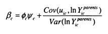

The first results I show in this section compare the estimates of changes in intergenerational mobility from the previous chapter with those which control for education. When controls for education are added to the intergenerational model
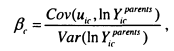

which is the extent of intergenerational persistence taking into account the impact of educational differences, this was referred to as ‘unexplained persistence ’ in Chapter 3. If unexplained persistence changes by less than overall persistence this indicates that education must be responsible for part of the increase in the relationship between incomes across generations.
In the context of the decomposition, y/c can be interpreted as a measure of educational inequality. This implies a linear relationship between education and parental income, but if one thinks more generally about the distribution of educational outcomes for people from different income backgrounds there are many definitions of educational inequality which could be used. Suppose we split the income distribution into q quantiles then we could compare education gaps across quantiles and look at how they evolve through time. I follow this approach in the empirical work in this chapter, and begin by looking at income quintiles (setting q = 5), and defining educational inequality as the gap in educational outcomes of those with parental incomes in the top relative to the bottom income quintile. To check robustness, I experiment with alternative measures of educational inequality in Section 5.5.
Descriptive Statistics
Table 5.1 shows the patterns of education and family income for the main datasets used in this analysis, the NCDS, the BCS and the BHPS. The first line gives information about the precise cohorts which are being compared in my analysis; obviously the NCDS and BCS are the 1958 and 1970 cohorts respectively. These cohorts were taking staying on decisions in 1974 and 1986 and would have potentially joined the higher education system in 1976/1977 and 1988/1989. The samples drawn from the BHPS are more complex as they are based on a number of birth cohorts and samples differ for the staying on and degree models. The sample used to find out about staying on was bom on average in 1979, and spans those bom between 1975 and 1984. This sample was aged 16 i.e. taking decisions about staying on between 1990 and 2001. The degree sample is older, including only those bom between 1974 and 1979 (the average year of birth is 1976.5), the sample potentially entered higher education between 1992/1993 and 1997/1998. The BHPS data therefore gives a picture of what is happening for those making decisions about post-compulsory schooling in the 1990s.
The education information displayed in Table 5.1 re-confirms the patterns shown in Figure 5.1. There is a strong rise in staying on and degree graduation by 23. Staying on rates increased from 40 percent to over 70 percent between 1974 and the late 1990s, while the proportion with a degree increased from 10 percent to 25 percent. The standard deviations of family income (given in parentheses) confirm the rise in income inequality which occurred for families with children over this time period.
Intergenerational Mobility and Education
To motivate the discussion of educational inequality I first show the contribution made by education to the changes in intergenerational mobility found in the previous chapter. This can be shown by comparing the change in unconditional measures of intergenerational mobility for sons39 with measures of the change which control for the fact that individuals differ in their educational attainments. To keep this investigation in line with the rest of the chapter the education controls added are whether the son stayed on at school past the compulsory age and if he attained a degree by age 23.
Table 5.2 shows the results of this exercise. Education does play a role in explaining the change in intergenerational mobility for sons as adding education variables to the model has a larger impact on the results for the BCS. The increase in the unconditional /? is .085 compared with .060 for the results conditional on education. The effect of adding education is similar for the partial correlation, the change reduces from .119 to .083. In both cases adding education to the model explains 30 percent of the rise in intergenerational persistence observed between the 1958 and 1970 cohorts. This suggests that a closer examination of the relationship between parental income and educational attainment is warranted.
The discussion of equation 5.4 above made it clear that education can explain intergenerational mobility through two routes: the relationship between parental income and education and the returns to education. The finding that education can explain the rise in intergenerational mobility could reflect either of these dimensions. In keeping with the results in the remainder of this chapter the education variables added are ‘stayed on beyond age 16’ and ‘degree attained’.
391 report results only for sons here to be consistent with the results from Chapter 4 and to avoid the difficulties in measuring intergenerational mobility for daughters; this will be returned to in Chapter 6. Results in Blanden, Goodman, Gregg and Machin (2004), which ignore these complications, find that education is responsible for even more of the change in mobility for daughters than sons.
There is evidence of a rise in the conditional return to degrees but a fall in the return to staying on. The strength of the positive relationship with parental income has increased for both these outcomes; this implies that a large part of increasing role of education in intergenerational persistence comes through the rising association between parental income and sons’ educational attainment. This suggests that a closer examination of the relationship between parental income and educational attainment is warranted40.
Educational Inequality
I begin my investigation of the changing distribution of educational opportunities by considering the evolution of staying on beyond the minimum school leaving age by parental income group. As discussed in the data section, I am able to examine this using longitudinal data from the cohort studies and the BHPS and using cross-section household data from the FES.
Table 5.3 looks at staying on rates broken down by parental income group over the three longitudinal data sources I use. Since the staying on decision occurs at age 16, the three periods in the spotlight are 1974 (for the 1958 cohort), 1986 (for the 1970 cohort) and 1990-2001 (for the BHPS individuals). The Table shows the proportion staying on beyond age 16 for people from the highest quintile, middle three quintiles and bottom quintile of the parental income distribution for these three data sources. Educational inequality is the gap in the proportion staying on between the highest and lowest quintiles. This is reported in the final column.
In all cases the gap between the staying on rates of those from the richest and poorest backgrounds are large, between 25 and 40 percentage points. Also, as has already been demonstrated in the aggregate figures, the Table shows there to have been a rise in the staying on rate for people from all parental income groups. What is interesting is the way that the distribution of this rise varies between income groups. Between 1974 and 1986 the largest rise occurs for young people from higher income groups (rising from .57 to .70) whereas between 1986 and the
40 When continuous ‘years of education’ variables are used in the decomposition, this result is even clearer, there is a slight downward shift in the return to schooling and a strong rise in the association between parental income and years of schooling.
1990s, the largest rise occurs for those from lower income groups (from .32 to .62). Consequently educational inequality rises by .11 between the first and second cohorts, and falls by .14 between the second and third cohorts.
Using the Family Expenditure Survey to match 17/18 year olds with their family income enables us to consider these changes in more year-on-year detail. The results obtained are given in Table 5.4. Again educational inequality is large at a given point-in-time with there being sizable differences in staying on rates between young people from high and low income backgrounds. The change over time is very similar to that found in the cohort data. Educational inequality was .28 for cohorts leaving school between 1977 and 1979. This rose to .40 in 1986- 1988, before subsequently falling back to .26 for those leaving school between 1998 and 2000. The pattern of changes is therefore very similar for both the longitudinal and cross-section data.
The time series pattern of these changes ties in very closely to the policy changes discussed earlier. As already mentioned, 1988 was the first year in which 16 year olds took the GCSE qualification; this also coincided with the beginning of the strongest period of growth in post-compulsory participation the UK has ever seen. It seems that the exam reform resulted in a weaker association between income and education under the GCSE system, where in most subjects all individuals are entered to take exams and more meet the standard acceptable to continue on in the schooling system41.
My results for post-16 participation indicate increased educational inequality up to 1988 and then a narrowing in educational inequality in the period after GCSEs were introduced. A key question is whether this continued through to higher education. One can make arguments either way here. Perhaps the school system matters most so that the increased staying on rates for people from poorer families ought to manifest itself in less inequality at HE level. On the other hand, the opportunity and direct costs of study are higher at older ages, and policy changes appear to have led to Government-funded student support being less
41 An alternative explanation is that young people were influenced by labour market conditions. I have investigated this, and mapping regional youth unemployment rates into the data does little to explain the changes.
targeted towards poor students. If this matters, one may not see inequality at HE level falling, even if it does at earlier stages of the education sequence.
Due to the data requirements, I am only able to explore these changes using the longitudinal sources: the cohort studies and the BHPS. Table 5.5 presents results for obtaining a degree by age 23 that are analogous to those presented for staying on in Table 5.3. The Table shows a large rise in higher educational inequality (from .15 to .30) between the 1958 and 1970 cohorts. This is consistent with increased educational inequality being in part responsible for the fall in intergenerational mobility observed earlier. However, in contrast to the results for staying on, educational inequality continues to increase through to the BHPS young people around 1999. As such, higher educational inequality has persistently risen in Britain since the late 1970s. Put alternatively, the expansion of higher education has more strongly benefited children from richer families.
The initial analysis of educational inequality presented above indicates that up until the change in the secondary examination system in 1988, increased opportunities to carry on studying at age 16 and 18 were being mostly taken up by those from richer backgrounds. After the GCSE was introduced, this trend reversed at age 16, with the staying on rates of the poorest youngsters beginning to catch up with their peers. This change was not seen for higher education attainment, where the gap between rich and poor continued to widen42.
There are a number of interpretations which can be placed on the growing educational inequality in higher education participation. One possibility is that it could be a consequence of the policies outlined in Section 5.2 which reduced students’ access to means-tested support. Earlier I described the policy environments faced by students in the different cohorts. What was very clear from this discussion is that the real value of means-tested grants declined over the period. This could therefore provide an explanation for the increase in educational inequality in higher education participation observed. However, my analysis suggests that larger changes in financial arrangements occurred over the 1990s than between 1976/1977 and 1988/1989, it is therefore surprising that the largest
42 It should be noted that the earliest years of data used from the BHPS refers to years during the large increases in staying on and HE participation shown in Figure 5.1, so the data will not fully represent the situation after these increases occurred. More work is needed to look at the most recent years of data as they become available.
increases in educational inequality in HE occurred between the first and second cohorts, rather than between the second and third. One hypothesis is that the changes over the 1990s affected the younger individuals in the BHPS most, and this impact is understated by the large range of birth years included in the BHPS data. Unfortunately, there is insufficient data to enable an analysis of differences through the 1990s, so this must be flagged up for future work.
An alternative explanation is that the disproportionate participation of those from higher income groups is a direct effect of the expansion in higher education. In particular, if young people with higher income are on average of higher ability then it would be expected that these would be more likely to take advantage of an increase in the number of places. Willen, Hendel and Shapiro (2004) construct a similar argument about the cost of college in the US, they argue that if education serves a signalling function then reductions in the cost of college will lead to a tighter link between ability and education; resulting in a rise in the college wage premium.
As mentioned above, Galindo-Rueda and Vignoles (forthcoming) consider the connection between ability and educational attainment in the British Cohort data. They find a declining relationship between attainment and ability, with those with lower ability and high parental income the group to improve their educational attainment by the most over time. The authors point to the end of selective education as one of the main drivers behind this change. The changes between the second and third cohorts would not have been influenced by the end of the selective system; and it is unfortunate that it is not possible to assess how interactions with ability influence the more recent results.
5.5 Robustness Checks on Educational Inequality
In this section I subject my findings on educational inequality to a number of tests. In many ways the analysis presented so far has been quite specific in terms of the sample used and the approach taken, here I experiment with the results in a number of ways to check that my conclusions do not change.
Results by Gender
To maximise sample size the results displayed so far are for pooled samples of males and females. We may wonder if the trends in educational inequality observed are consistent across genders, especially as the results I have shown for the impact of education on intergenerational mobility are for sons only. This concern can be dismissed as separate analyses reveal that while participation rates vary by gender (girls are more likely to stay on at school) there are very similar overall trends in educational inequality for males and females. For example, over all three cohorts educational inequality in higher education completion rose by .22 for men from .16 to .38 while for women it rises by .23 from .14 to .37.
Measurement Error
Throughout this thesis I have stressed the difficulties caused by imperfect measures of parental income and the same argument applies here. Theoretical models of parental investments encourage us to think that permanent income through childhood is what matters for educational attainment. In the models presented I am limited to using one-shot measures of parental income, which will be poor estimates of permanent income, and will lead to a downward bias on educational inequality. As the focus of this research is to look at changes over time, this attenuation bias will only matter if it is not constant.
The FES provides one way to check the effect of attenuation which is not available in the other data sets, as it has information on family expenditure as well as income. I treat consumption as a proxy for permanent income, this follows Friedman’s permanent income hypothesis (1957), which states that individuals will make consumption decisions on the basis of permanent rather than current income. Consumption has also been exploited as a proxy for permanent income in Blundell and Preston (1998).
Table 5.6 compares results for staying on inequality based on family consumption quintile with those based on income quintile shown previously. It is clear that using consumption data does reduce the downward bias on the results. In every case the estimates of educational inequality are larger when consumption quintiles are used rather than income quintiles. The overall trend from the income data is that educational inequality is widening significantly up to 1986-88 and then narrows significantly in the remaining periods up to 2000. The consumption data reveals the same trend, but more muted, as neither the rise or fall in inequality is statistically significant. This seems primarily to be driven by the result for 1986-1988 which appears to be less affected than other periods by whether income or consumption is used to generate the quintiles.
Alternative Specifications
For the results discussed up to this point educational inequality has been defined as the difference between the participation or attainment of the richest quintile compared with the poorest quintile. As already noted, this is just one possible way of finding out how the relationship between education and parental income has changed over time. In this section I check if similar changes are observed for alternative measures, using quartiles, deciles and finally a linear relationship between education and parental income (the relationship implied by the decomposition).
To ease computation these measures are derived using Probit models rather than by comparing the proportions in each income group. The results from the Probit models which show educational inequality by quintile are precisely comparable to those obtained from the descriptive methodology, as we shall see. The additional advantage of using econometric models is that it is straightforward to add controls. This will be exploited when I try to identify the causal relationship, but in this section no controls are added.
To reiterate, the educational outcomes of interest can be represented as a 0-1 dependent variable in a Probit model, where the explanatory variable is some function of parental income.
![]()

A quintile specification, such as has been used so far, amounts to estimating
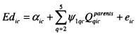

Where the Q ic variables are dummy variables for parental income quintile q in cohort c, leaving out the lowest quintile, q= 1.
Measures of educational inequality equivalent to those shown earlier can be derived from this model as the marginal effect on the probability of the outcome of having parents in the richest quintile rather than the poorest quintile.

where 3>(.) is the standard normal cdf. Standard errors for this measure are obtained by bootstrapping.
This model is easily transferred to the quartile and decile specifications by changing the number of quantiles to q=4 and 4= 10. The measure of educational inequality in these cases will be comparing the education of those in the top and bottom quartile of parental income and in the top and bottom decile of parental income. I also present models which use log income as the explanatory variable. The interpretation of the linear models is that a marginal effect of income on staying on of .2 implies that a 10 percent increase in parental income is associated with a 2 percent rise in the probability of staying on.
Table 5.7 reports results on changes over time in educational inequality based on alternative income specifications. The upper panel does this for staying on beyond the minimum school leaving age, while the lower panel shows results for degree attainment at age 23. These results show clearly that when educational inequality is calculated on a finer gradation, observed educational inequality rises. Measured inequalities based on deciles are larger than those based on quintiles, which in turn, are larger than those based on quartiles. This is expected, as a positive correlation between income and attainment implies that the top decile will have more education than the top quintile and the bottom decile will have less than the bottom quintile.
Reassuringly, patterns over time are similar across all the specifications; there is evidence of a rise in the relationship between income and staying on in the first period from the NCDS to BCS, followed by a fall between the BCS and BHPS. While there is some evidence that the initial rise in inequality in the first period may be weaker under alternative specifications the fall in inequality after 1986 is clear whatever specification is used. In all cases the result that inequality in HE completion has increased over the three periods stands.
5.6 Methods to Establish Causality in the Relationship between Parental Income and Education43
The results from the preceding sections confirm that educational participation and attainment is strongly related to parental background. Those from richer families have a much greater chance of success than their poorer peers. If a goal of Government policy is to narrow these gaps then it is essential to understand the mechanisms behind them. In this section I move away from the descriptive analysis undertaken so far to attempt to identify the causal relationship between parental income and education.
The fundamental question is whether it is money itself which is generating the differences in attainment between those from different family backgrounds. This is particularly crucial for understanding if redistribution or reductions in child poverty can lead to a narrowing in educational inequality. If the drivers of educational inequality are ability, parental education, parental motivation etc. then changes in the distribution of income will have no effect on the extent of educational inequality. However, if parents use income to make investments in child care quality, the home environment and educational activities then we would anticipate that increases in parental income would have a real benefit for children’s educational outcomes. Gregg, Waldfogel and Washbrook (2005) support this interpretation by showing that income gains for poor parents are spent disproportionately on children’s goods such as children’s clothing, books and toys.
Taking the earlier model of educational attainment, and expressing it in a linear form, enables a more formal explanation of the identification problem. However, the parameter of interest is no longer \f/, but is 0, the causal impact of parental income on educational attainment. As I am no longer interested in changes between cohorts the subscript c has been dropped, however education and
43 This section and the one that follows it are a shortened and revised version of the work
presented in Blanden and Gregg (2004).
parental income now vary with time for individuals so a subscript t has been added, this becomes important later in this section.
![]()

Educational attainment is a function of many variables ( A,t), both observed and unobservable, which influence child attainment. The difficulty arises because the cov(Ait,Y*H,ren’s) > 0 , consequently estimating 9 from equation (5.8) will lead to an upward biased estimate of the effect of parental income on education.
A typical starting point to solving this identification problem is to control directly for the factors which lead to differences in educational attainments, and are positively correlated with income. These include parental education, unemployment, family status and child ability. Gregg and Machin (2000) present an analysis along these lines and find that significant parental income effects remain when many controls are added. The difficulty is that \ will consist of both observable characteristics, X it and unobservables Z(. When controls for X it are added an upward bias will persist if there is a positive correlation between Z. and Y^arents.
The most convincing way to disentangle the impact of unobserved heterogeneity is to use data from experiments. In the simplest form this would involve giving some families additional income while the income of other families remained unchanged, and then measuring the impact this had on children’s attainment. With a proper design, the income change will be unrelated to differences between children and their families (Zf).
It may be difficult to imagine a setting where such an experiment could take place, however two programmes in the US have come close. States administering welfare to work programs in the late 1990s were entitled to add an evaluation aspect which involved randomising treatment, while the Moving to Opportunity44 projects all had a randomised approach. Fortunately child outcomes
44 The Moving to Opportunity Projects selected families in poor neighbourhoods into three groups: the first group has help with rents provided they move to a more affluent neighbourhood, the second group has help with rents to move to any neighbourhood while the third group receives no assistance.
were part of the evaluations of both programmes. However, in both programmes the intervention is not simply giving families more income. For the welfare to work programme, cash only comes when mothers move into work (although this can be accounted for by comparing with mothers who are also helped to move into work but receive no income supplement). The Moving to Opportunity programme can be used to discover how income may work through just one channel; neighbourhood quality.
Clark-Kauffman et al (2003) summarise what can be learned from the welfare to work evaluations while Goering and Feins (2003) do the same for Moving to Opportunity. Welfare to work programmes are shown to have significant positive effects on the test scores of pre-schoolers while Moving to Opportunity is shown to have a number of positive benefits for children in terms of test scores, behaviour and reducing criminal behaviour. These studies, therefore, provide powerful evidence for income effects on child outcomes; however the specific samples involved and the enforced link between income increases and other changes may mean that the results do not generalize to the population at large.
A more feasible alternative is to use instrumental variables (IV) to identify income effects. This requires a variable which influences parental income without having a direct effect on children’s education; a tall order. Shea (2000) and Chevalier et al (2005) use parental union status as their instrumental variable, on the grounds that this leads to higher parental earnings through additional rents, but that this is uncorrelated with other characteristics. Chevalier et al’s results for the UK indicate that parental income effects are much larger using this IV approach; a counter-intuitive result.
Instrumental variable approaches appear to be more successful in discovering the causal impact of parental education on children’s outcomes. Chevalier (2004), Chevalier et al (2005), Oreopoulos et al (2003) and Black et al (2005a) have all used changes in compulsory schooling laws to identify the effect of an increase in parental education on children’s attainment. The results for the UK from Chevalier and from Oreopoulos et al for the US, imply that the causal impact of parental education is strong while results for Norway in Black et al reveal only weak effects of parental education. The limitation of all these analyses is that they are local average treatment effects, which will only apply to those parents who take more education as a result of the change in the law.
In cases where experiments are not available and convincing instruments cannot be found, approaches can be used which rely on variations in income within the household.
The model of attainment and income with controls added is
![]()

It is therefore the correlation between Z, and which generates the upward bias. The principle behind sibling fixed effects models is to assume that Z( is equal across siblings, or put alternatively, that the sibling specific part of the error (uit) is uncorrelated with parental income. The sibling fixed-effects model is estimated on deviations of Edit and Yit from the family mean; this eliminates the impact of Z( and generates unbiased estimates of 6 .
The variation in family incomes experienced by the siblings comes from the age gap between them. This means that siblings will be affected by income in different periods because other children have either not been bom yet or have already left home. This approach uses income variations within a family rather than differences across families. Sibling studies require an income history for the family including some periods of differing income experience.
The central problems for sibling studies is that siblings will often be close in age and experience very similar income patterns for most of their childhood. Further, taking differences increases the attenuation bias due to measurement error in data reporting. An additional problem emerges from new findings in Black et al (2005b). This paper discusses how educational outcomes may vary by family size and birth order. Differences by family size may mean that results are not generalizable across different family sizes as only families with two or more children can be used in sibling-difference estimations. Differences in attainment by birth order lead to even greater difficulties for this estimation methodology as sibling-specific errors will not be random across birth-order. If families grow richer over time and (as Black et al suggest) older children tend to be more
successful, this will lead to a downward bias on the measured income effect.
An advantage of the sibling-difference approach is that income shocks in the family will be experienced by siblings at different ages; this can provide evidence on when in childhood income matters most. Levy and Duncan (2000) describe a recent sibling study using the Panel Study of Income Dynamics. They find that parental income matters most for young children but that the magnitudes of the effects are small with a 2.7 fold increase in family income through childhood adding three quarters of a year to completed years of schooling by age 20. These are extremely small impacts compared with others found in the literature.
Mayer (1997) adopts an alternative route to control forZ,. Leaving aside the question of measurement error, income at a point in time can be thought of as composed of transitory and permanent components.
![]()

Therefore in a regression of the relationship between income and education the income parameter will be a weighted-average of the coefficients that would be obtained if measures of permanent and transitory income could be entered into the model separately. The key assumption here is that the bias is generated by the correlation between Z. and the permanent component of income. The transient income component is assumed to be uncorrelated with fixed family characteristics so thatcov(l'”wu ,Z ,) = 0, and therefore the coefficient on Yilrans would be the true relationship between parental income and education. The strategy is to use a measure of family income after the child has completed the normal education process as a control for the permanent component of income. The estimation equation thus looks like
![]()

Any correlation between the later income measure and attainment is not causal and its inclusion can be seen as an attempt to condition out the permanent income component. If Yu+i was perfectly correlated with Y?erm then 6 would be the relationship between education and transitory income at age 16. However, Yit+l also contains a transitory component, meaning some residual bias will remain in this approach. This can be reduced by averaging over several years of later income.
Mayer uses a range of child outcomes and test scores as dependent variables. The addition of post-childhood family income reduces the estimated impact of a 10 percent increase in income on years of schooling from 1.86 to 1.68 (after conditioning on observed family fixed characteristics). The conditioning on later income makes only a minor difference to the years of schooling results but is more important for other outcomes such as teenage motherhood and dropping out of school.
There are several concerns with this approach. The first is that income changes between the two periods considered may reflect family shocks that influence child attainment independently. In addition, lifecycle models predict that anticipated income changes will affect behaviour in all periods if families can smooth consumption. The final, and most damning, problem is that the investment model which underlies these estimations is firmly couched in terms of permanent income not transitory income. By conditioning for permanent income, all the variation of interest may be lost. Indeed, this difficulty also applies to the sibling model, as mean family income is differenced out. This means that the estimates of the effect of parental will be downward biased, giving more confidence in any significant results which are found.
5.7 The Causal Impact of Parental Income on Education in the UK
The evidence from US data implies that there are significant, although possibly small, impacts of parental income on educational attainment. In the final empirical contribution made in this chapter I use some of the techniques described above to investigate the extent of the causal relationship between parental income and educational attainment in the UK.
Adding Controls
I begin by assessing how the patterns of change over time are modified by taking the most straightforward approach to reducing bias; adding controls to the models. To be consistent with what has gone before, I show the impact of adding controls to models of educational inequality based on quintiles. In the upper panel of Table 5.8 I show models for the NCDS, BCS and BHPS for staying on while the lower half of the table reports the same models for degree attainment.
The first specifications (A) in each table show the results with no controls for comparison purposes45. The remainder of the specifications add additional controls for family background and the individual characteristics of the child. Specification B focuses on accounting for the impact of family structure by controlling for the child’s sex, the number of children in the household, parents’ age and the absence of a father figure. Specification C focuses on controlling for parental education, one of the main aspects which might be related to child attainment and correlated with family income. In the final models I am able to use information on test scores to take out the relationship between child ability and parental income; although this is only possible for the first two time periods as test scores are not available in the BHPS.
The results for the three cohorts show that the relationship between parental income and educational attainment can be somewhat explained by the controls I add, but that significant income effects remain. The controls for parental education are particularly important in reducing the estimates. Observed educational inequality is 40 to 50 percent lower when controls for mothers’ and fathers’ education levels are added. Adding controls for child’s ability at ages 11/10 further reduces the estimates. For the NCDS, the estimate of educational inequality for degree attainment falls from .146 with no controls to .036 with controls for family structure, parental education and ability.
For the first two time periods adding controls to these models has very little effect on the patterns of changes over time, for both dependent variables the rise in educational inequality is robust and remains significant under the most stringent models. The same is not true for the later change, which compares the results from the BCS with those from the BHPS. The first two models in the lower panel of Table 5.8 show that there is a strong (although insignificant due to the sample size), rise in educational inequality at degree level for those entering university around 1988/1989 and those entering from 1992/1993 through to
45 For the BHPS these results differ slightly from those in descriptive statistics as I have added controls for birth year and wave observed.
1997/1998. When parental education is added to this model educational inequality appears flat over this period. This implies that the change over the 1990s can be explained by the children of higher educated parents doing better, rather than a change in the causal effect of income.
The discussion of identification methods highlighted that adding controls to models of the education and income relationship will not suffice if there remains unobserved heterogeneity correlated with parental income. To provide more convincing evidence, I now experiment with sibling fixed effects estimators and adding controls for permanent income. Due to the data requirements of these approaches I am only able to use the BHPS; fortunately this is the most up to date of the data sources used here.
Sibling Fixed Effects Estimators
The results of the sibling models for the BHPS are given in Table 5.9. Due to the shortness of the panel we do not observe family incomes and full education histories for all siblings so the results for different qualification levels use slightly different samples of individuals.
The upper panel of the Table shows marginal effects for a linear probability model of staying on and income at age 16. In all cases I control for family structure as described in the notes to Table 5.8 (sex of the cohort member, number of siblings, parents’ age) as well as controlling for both parents’ work status when income is observed, as this may be correlated with both income and performance. First, I show the impact for this model of only focusing on a sample of siblings (column 2) rather than including single child families (column 1) where both models include basic controls for family structure. Limiting the sample to siblings makes very little difference. In the third column I show equivalent models to those in the previous section by adding controls, including parental education. As before, this brings down the estimate; from .107 to .069. The final column reports estimates from the sibling fixed effect models. This does not reduce the marginal effect by as much as simply controlling for parental education, the coefficient for this model is .079. The disadvantage of the fixed effect approach is that the fall in the signal to noise ratio leads to a rise in the standard errors leaving the income coefficient significant at only the 10 percent level.
The lower panel uses degree attainment as the dependent variable. In this case the explanatory variable used is parental income at age 18. This seems appropriate as this is the age when university enrolment choices are made for most young people. In addition, choosing a measure of income obtained closer to the outcome increases the available sample size. For this model the income effect changes more between the full sample and sibling sample, it is higher for those with siblings in the sample46. The marginal effect of income on the probability of degree attainment is .162 with basic controls, and .090 in both of the models which attempt to account for unobserved heterogeneity. The difference is that the standard error is inflated for the sibling fixed effects models.
The results of these modes indicate that sibling fixed effects estimates of the impact of parental income on education are the same or slightly larger than those which simply control for parental education. The implication of this is that there is no additional upward bias to remove once parental education is controlled for. However, this is a strong conclusion to draw given the size of the estimated standard errors. The large standard errors are due to the main limitation of sibling estimation; relying on differences in income within families for identification enhances the effect of measurement error and reduces the variation in income and outcomes that can be used to identify effects.
Controlling for Permanent Income
Table 5.10 explores Mayer’s approach of adding post-education income to the model, using data from the BHPS. This is an attempt to control for permanent income, thus removing the correlation between parental income and unobserved heterogeneity. In choosing the age at which post-childhood income is observed I must balance two factors. First, income must be taken at an age sufficiently removed from the educational process to satisfy the assumption that it will not be
46 To be included here siblings need to be fairly close together in age as income and outcome variables are further apart in time. This may explain the stronger results for the sibling sample as it seems plausible that income constraints on university attendance are more important for parents who are contemplating sending two or more children to university in quick succession.
correlated directly with educational outcomes. However, sample size considerations also play a role; the further away the income is from the outcome of interest the smaller the sample size will be. I show results conditioning on just income at age 20 and on an average of income between 18 and 21. Ideally I would wish to use income at later ages but sample sizes become prohibitively small if this is attempted.
I show Probit models for the two outcomes of interest, staying on and degree attainment by age 23. All models control for parental education. For both dependent variables the impact of adding controlling for age 20 incomes is limited while adding average income from age 18-21 reduces the impact of income rather more. This is anticipated as the three year average will be a rather better estimate of permanent income. In the model with controls for parental income the marginal effect of income is .112 for staying on and .175 on degree attainment. These effects reduce to .080 and .146 when average income between 18 and 21 is controlled for.
For both models this approach indicates that upward bias is further reduced by controlling for a proxy of permanent income. The marginal effects fall by 20 to 30 percent using this method, compared to controlling simply for observed characteristics.
Summary
Discovering the causal relationship between parental income and educational attainment is a difficult identification problem. I would not claim that the methods proposed here are perfect, but nonetheless some lessons can be learned from my investigation. The main conclusion is that adding controls makes a big difference to the levels of educational inequality recorded. Adding controls for parental education, in particular, reduce the observed educational inequality by around 50 percent; it is clear that parental education confers a strong advantage, which could not be overcome by redistribution. In addition, some of the impact of parental education is mediated by early ability, this supports the Government’s policy programme of concentrating on early years’ education to help children get a good start in the education system. The methods which rely on removing the permanent effects of unobserved heterogeneity do not reduce the estimates much further. Therefore, as far as we can tell, there is strong evidence to suggest that there is, at least, a small causal impact from parental income to educational attainment47.
5.8 Conclusion
Reducing the link between parental background and educational attainment is seen as one of the main ways in which Government policy can help to reduce intergenerational inequalities. The empirical results set out in this chapter have a number of important contributions to make to the academic and policy debate about the contribution of made by educational inequalities to intergenerational persistence.
Thirty percent of the fall in intergenerational mobility for sons can be explained by changes in access to education, in spite of the fact that educational opportunities for young people as a whole were improving over this time period, with increases in participation at both post-compulsory and higher education. A more detailed examination of patterns of participation by parental income group reveals that the children of higher income parents benefited disproportionately from the expansion in higher education. Their participation rose much faster than that of poorer young people. The most recent evidence does not suggest that this situation has reversed up to the end of the 1990s.
These findings do not present a very reassuring picture for future social mobility in Britain. The current Government policy is to encourage further expansion in the proportion of young people attending University, but previous expansions appear to have only exacerbated the gap in access by family background. In addition, we may worry that the introduction of student fees will only worsen this trend, although the expansion in the level of mean-tested assistance and discretionary assistance from Universities may suffice to counter
47 In order to keep this section of a reasonable length I have shied away from fully interpreting the magnitudes of the effects I find. However, evidence from Blanden and Gregg (2004) suggests that a £140 increase in income per week (in 2000 prices) raises the probability of obtaining a degree by 4 percentage points using the best estimates from causal models while non-causal models suggest that a £140 difference in weekly income is associated with a 9 percentage point difference in the probability of obtaining a degree.
he impact of fees. It will be important to repeat the analysis carried out in this chapter to evaluate the impact of the forthcoming changes.
The current direction of Government policy is to address educational inequalities at early ages, mostly through specific educational programmes but also by raising the living standards of poor families. My efforts to identify the causal effect of parental income on educational attainment are an attempt to evaluate the relative impact of these types of policy. While there are significant causal effects of parental income on educational attainment, it seems that redistribution alone will only be able to close a small part of the large education gap, for the rest we must turn to more direct interventions.

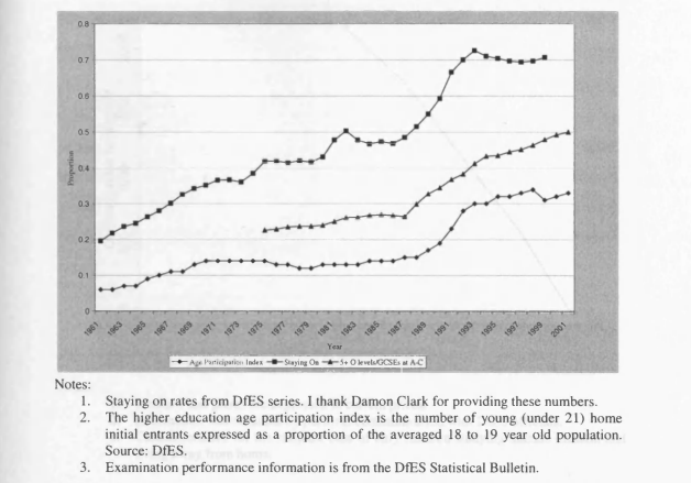

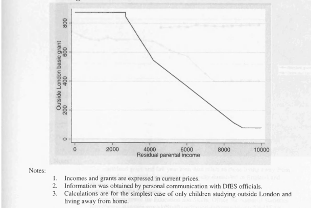

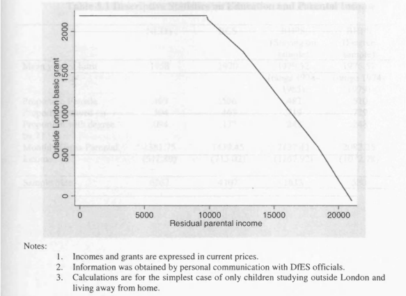

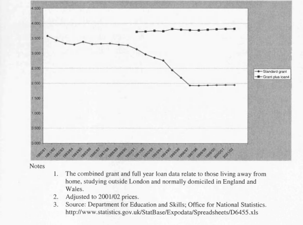

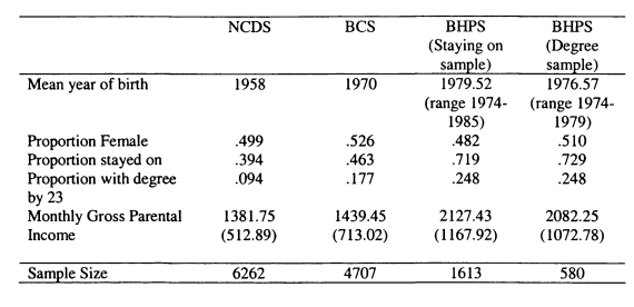

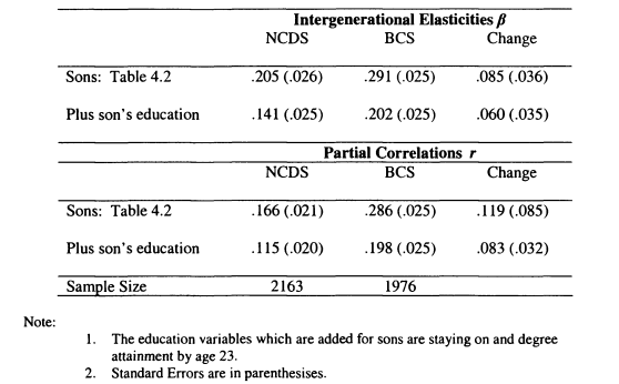

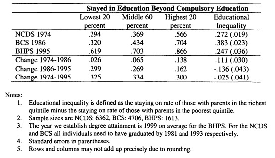

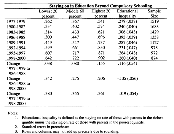

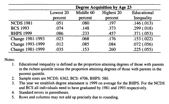

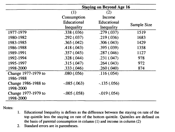
Parental Income Relationships

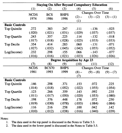
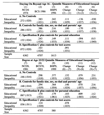

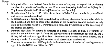


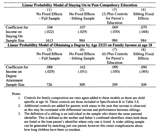
Controlling for Sibling Fixed Effects using the BHPS

Controlling for Permanent Income using the BHPS
Chapter 6: Intergenerational Mobility and Assortative Mating in the UK
6.1. Introduction
This thesis considers the links between economic status across generations. So far, I have considered this question solely in terms of the relationship between parental income and individual earnings and education levels. It seems natural to think that household income is a better measure of economic welfare than individual earnings when households pool income and benefit from economies of scale and household public goods. Indeed, poverty is usually measured at the household, rather than at the individual level. Economic status for those in couples is therefore substantially influenced by their partners’ earnings. In this chapter, I broaden my focus to consider the role of partners’ earnings in contributing to the intergenerational links within families. If assortative mating is strong, the persistence of family incomes across generations might be stronger than is observed based on individual earnings.
As reviewed in Chapter 2, previous economic research on the interaction between intergenerational mobility and assortative mating is limited. All the studies that have been carried out suggest that partners contribute substantially to intergenerational persistence (Solon and Chadwick, 2002, Ermisch et al 2004, Lam and Schoeni, 1994). The only previous estimates of income mobility and assortative mating in the UK are found in Atkinson (1983), which suggests that assortative mating is very strong. Indeed, the relationship between the earnings of fathers and sons-in-law’s earnings is stronger than that found between fathers and sons. More recent estimates from Ermisch et al (2004) are based on occupational indices; in this respect, the relationship between fathers and sons-in-law are lower than between fathers and sons, but still substantial.
In Chapter 4 I have demonstrated, based on individual measures, that intergenerational mobility in the UK has fallen when comparing sons bom in 1958 with those bom in 1970. Here I examine whether these changes are replicated for daughters’ earnings and once the partners of both sons and daughters are added to the picture. The consideration of sons and their partners and daughters and their partners symmetrically is an innovation in this chapter.
The previous literature has focused either on the persistence between sons and their parents or sons and their parents-in-law, largely playing down the role of women’s earnings. This is because the intergenerational mobility of women’s earnings is difficult to measure, as women participate in the labour market less often than men, and when they do, they often work part-time. In some ways this problem can be ignored, if we want to know about intergenerational earnings persistence at a point in time it is reasonable to simply measure this without taking account of selection issues. In fact, measuring the way in which intergenerational mobility changes as patterns of female participation alters is an important focus of this chapter. However, as we have seen in Chapter 2, the theoretical background to these models is firmly couched in terms of permanent income. Therefore, I investigate how the results are being affected, and possibly distorted, by participation decisions.
I begin this chapter by reviewing the theoretical background to intergenerational mobility and assortative mating first discussed in Section 2.5. This demonstrates why persistence between an individual’s parental income and his or her partner’s earnings may vary. The conclusions of this simple approach are clear; the link between parental income and partner’s earnings is increasing with the strength of assortative mating. If assortative mating is strong, the elasticity of partner’s earnings with respect parental income will be similar to that for the child’s own earnings.
In my results, I estimate the relationships described in the model to build up a picture of how assortative mating and intergenerational transmissions are related. I first develop a picture of how individuals match by education level. I find some evidence that assortative mating has increased. I also consider the relationship between parental income and the education of partners; these relationships are strong in all cases, pointing to substantial assortative mating. However, I find less evidence of change for these estimates.
The most important set of results show the regression coefficients and correlations between the earnings of sons, daughters-in-law, daughters and sonsin-law and their parents’ (or parents-in-law’s) income. I find, as expected, that the correlation between partners’ earnings and parental incomes are strong. The most interesting results show that these relationships have changed quite substantially, especially for the earnings of daughters-in-law. In the earlier cohort, there was only a very weak relationship between daughters-in-law’s earnings and parental income, whereas in the later cohort this is as almost as strong as the relationship between sons and their parents. There is a smaller, but still significant, increase in the relationship between daughters’ parental incomes and their partners’ earnings.
The challenge is to interpret these results. As emphasised above, we want to understand both the importance of changes in the underlying relationships and changes in the selection into employment. I therefore compare my uncorrected estimates for the employed sample with those which correct for the selection into employment. I find that in the second cohort, women’s participation decisions are more strongly correlated to their potential wages. This introduces an upward bias on the change in intergenerational elasticities when women’s eamings are the dependent variable. Indeed, this change in the selection into employment is in part responsible for the rise in the relationship between the eamings of daughters-inlaw and the parental income of sons.
In the next section, I present the theoretical background and measurement approach used in this chapter. Section 6.3 describes the data, particularly focusing on the changes in household formation and employment between the two cohorts. In Section 6 .4 ,1 discuss how the cohorts match by education level while Section 6.5 considers the relationship between parental income and the education levels of the next generation. In Section 6.6, 1 present my main results on intergenerational mobility, and show how they are influenced by changes in participation. In Section 6.7, I discuss the interpretation of my findings while Section 6.8 concludes.
6.2 Theoretical Background and Measurement Issues
Theory
The theoretical framework behind the relationship between intergenerational mobility and assortative mating has been discussed in Section 2.5. Here I take the model used in Ermisch at al (2004), where assortative mating occurs on the basis of human capital. In Lam and Schoeni (1994) and Chadwick and Solon (2002) mating occurs on the basis of full income. Simplifying the matching process to operating only on human capital serves to reduce the number of parameters relevant to the model and seems a reasonable summary of the literature on assortative mating.
Assortative mating is modelled as a , the positive correlation between the human capital of wives ( H wi) and husbands ( Hhi).
![]()

For both husbands and wives income is positively related to human capital, although the return to human capital may vary across gender as in equations (6.2) and (6.3) below.
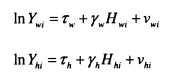

In this formulation the intergenerational relationship is driven by the optimising behaviour of parents. The parental utility function includes parental consumption and the child’s household income, so that the child’s partner’s income is also included. However, this does not affect the general conclusions of the model which are similar to Lam and Schoeni (1994) where the mechanism behind the correlation of education across generations is left ambiguous.
Parental utility is described in equation (6.4) where n indicates the extent to which parents are altruistic and care about their child’s income. From now on I shall express the model in terms of the wife’s parents’ income, so that parameters and variables relating to the parents are subscripted w . However, the model is fully symmetric for husbands and wives. I am assuming that all children marry.
![]()

Parents solve this model subject to their budget constraint. In this model, debt and bequests are not permitted, so that parents must spend all their available income on their own consumption and on the education of their children. Each unit of human capital has a price pH. Solving the model gives the following solution for the intergenerational parameter,/?, the coefficient from a log-log regression of child’s income on parental income.
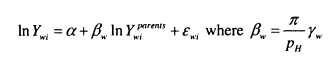

Intergenerational persistence for daughters is therefore positively related to parental altruism and the returns to education for women, but negatively related to the cost of investment.
Similar factors are important for the relationship between the husband’s income and his wife’s parental income. In this case, the male return to education is important and the relationship is moderated by assortative mating and the difference in the distribution of education between husbands and wives.
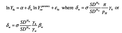

Putting /?and 8 together enables us to understand more about the expected relationship between these two parameters. If the model is worked through in terms of son’s parental income, the relationship is symmetric so that:
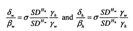

As shown, if the returns to education and the distributions of human capital are equal for men and women, the ratio of Sw and J3W, will enable the identification of a ; the elasticity between the income of the daughter’s partner and her parents’ income over the elasticity of her own income with respect to her parents’ income will be equal to the extent of assortative mating. In this chapter, the focus is on how these relationships change across cohorts. The implication of equation (6.7) is that increases in /? for sons (as observed in Chapter 4) are likely to lead to increases in S for daughters-in-law, ceteris paribus. In addition, increases in cr will lead to a rise in 8 relative to /?.
It is also clear that changes in the returns to human capital for men and women have a part to play in this model. If we think of the incomes in this model as permanent, participation will influence the return to human capital over the lifetime. The implication is that if daughters participate more, yw will increase and will rise relative to Sw, and ^ w ill rise relative to flh. This provides an illustration of how changing patterns of participation can influence intergenerational mobility. Of course, it is difficult to observe the implications of these lifetime factors when incomes for the children’s generation are observed at only one point in time.
A further implication of the model is that in order to understand changes in the relationship between parental income and partners’ eamings, it will be necessary to try to unpick changes in assortative mating ( a ) and changes in returns, which, as noted, may come through changes in participation. To express this in another way, if the association between daughters-in-law’s eamings and parental incomes increases we want to know if this is because individuals have changed the way they match or if the match has remained the same but wives’ working patterns have changed.
Measurement Issues
In the empirical work in this chapter, I estimate four parameters, j3h and Sh, based on regressions of eamings on parental income. I report partial correlations alongside these coefficients, as previously. Obtaining good estimates of these parameters has all the usual problems associated with measuring intergenerational mobility, which have been discussed throughout this thesis. However, lower participation and part-time work among women creates additional problems in estimating /3w and Sh, and I shall focus on these here.
The classic analysis of the problems caused by selection bias is presented in Heckman (1979). There are two equations governing the processes, an eamings equation for all women (where, in this case, the explanatory variable would be parental income) and a latent variable relationship governing the decision to participate.
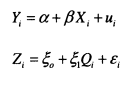

The woman participates only if Z, >0. Therefore the regression of the observed Yi on X, will be biased by an additional error term, similar to an omitted variable bias. If those with higher eamings are more likely to work, and X(is positively correlated with eamings, /? will be upward biased.
![]()

As always, it is the change in the selection bias which will be important when making comparisons across cohorts. In recent papers, Mulligan and Rubinstein (2004, 2005) discuss the implications of the changing selection of women into work for the gender wage gap. They argue that as the returns to skill have increased, potential wages have become increasingly important in determining the selection into work, leading to an increasing positive selection bias and an observed reduction in the gender wage gap. It is clear that selection bias may have changed for the daughters and daughters-in-law I observe in my data, particularly given the changes in characteristics across cohorts which I highlight in the data section. It is therefore necessary to attempt to model the influence of endogenous selection.
Heckman’s framework provides an obvious route to exploring the implications of the changing selection into work. The bias in equation (6.10) can be shown to equal
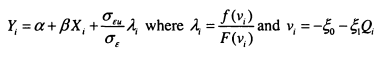

The bias will be larger the stronger is the correlation between the unobserved determinants of wages and participation. Inclusion of the inverse Mills ratio ( ) , demonstrates that the selection bias will be stronger when participation is low. While the extent of the bias can be estimated by making distributional assumptions it is more convincing to estimate the parameters of the correction using a Probit model of employment. In order to do this, it is necessary to have an exclusion restriction (i.e. a variable which determines employment but not eamings), so that the employment equation can be identified separately from the eamings model.
In their model of intergenerational occupational mobility, Ermisch et al (2004) account for the selection of women into work by incorporating a Heckman selection correction in their estimates. Ermisch et al use a number of variables to predict employment and then use the cubic of the predicted probability of employment index generated to identify the selection. I follow their approach, although acknowledge its limitations in my discussion of the results.
Heckman’s correction is very powerful as it provides a point estimate of the parameter of interest in the context of missing information. However Manski (forthcoming inter alia) believes that the distributional and exclusion restrictions invoked by this approach are too strong. In Manski’s formation each woman in the sample is characterised by(y,x,z), where yis the dependent variable (the woman’s permanent income), x is the explanatory variable (either her own or her husband’s parents’ incomes), z is a binary variable which takes the form of 1 if the woman is employed and 0 if she is not working. The regressions that are being estimated aim to reveal the relationship between y and jc , (E[y | jc] ) for the full sample of women. The law of total probability implies that
![]()

In other words, the true parameter will be a weighted average of E[y \ x, z = 1] and E[y | x, z = 0], where the weights depend on the proportion of women who are not working. There is no information which can identify E[y | jc, z = 0] and therefore one cannot identify a point estimate of E[y | x ]. Again, it is clear that the problem is exacerbated if a large proportion of the sample is not working.
Manski has developed a method to partially identify E[y | jc] by using the information that is available to derive bounds for the expected value. Minicozzi (2002) considers the intergenerational mobility of women using this approach. Initally she calculates the ‘worst case’ bounds, assuming no information is available about eamings for those not working full time. Minicozzi then narrows the bounds by making assumptions about the upper and lower bounds of eamings for individuals according to their characteristics and current work status. Unfortunately the bounds which result from these assumptions are still wide at .12 to .53. Having such wide bounds would make it very difficult to draw conclusions on the relative magnitudes of /? and£, which is why I prefer to use Heckman’s
approach.
I present results which show the uncorrected regression coefficients for the sample of employed individuals and also results which correct for selection. Both are informative. The uncorrected estimates will show how parental income is related to the eamings of daughters and daughters-in-law with the current patterns of employment. However, the selectivity corrected results enable me to try to separate the influence of changes in the selection into employment from changes in assortative mating.
An additional way of exploring the influence of assortative mating versus changes in participation is to estimate some of the other parameters from the model for the full sample. To begin with, I measure the relationship between the educational attainments of partners, as a direct measure of a for the two cohorts. Of course, couples will match on broader measures of human capital than educational attainment, so this will not provide a perfect estimate ofcr. An advantage of using education is that it is observed for the full population.
An alternative approach recognises the fact that matching and intergenerational investments are both modified through human capital. If we return to the model, it is clear that it also yields strong predictions about the relationship between human capital and parental education.
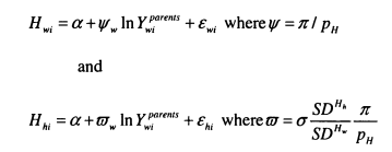

Consequently the relative magnitudes of y/ and crwill be informative about the extent of assortative mating. Again, this relies on the premise that the measures of educational attainment used here are good proxies for human capital.
6.3 Data
The data sources for the empirical work in this chapter are the same as those used in Chapters 4 and 5, the National Child Development Study (NCDS) and the British Cohort Study (BCS). I rely once again on the incomes of the cohort members’ parents at age 16 as the explanatory variable. This variable has been discussed extensively in Chapter 4, and the same caveats apply here. As a single piece of information on income is being used to proxy for the permanent income of parents, we must once again assume that the bias introduced is similar for both cohorts.
Information about the eamings of cohorts is available at age 33 in the NCDS (1958 cohort) and at age 30 in the BCS (1970 cohort). At the same time, information was obtained about the cohort member’s partner, for both married and cohabiting couples. I use the questions on partner’s sex (I drop the few same sex couples in the sample), partner’s age, employment status, education and eamings. As information is only available on partner’s net eamings, I also use the net eamings of cohort members, rather than the gross eamings measure used in previous chapters. The education variable available for partners is not very satisfactory – we only know the age at which partners completed their full-time education. This is much less useful than the variables detailing qualification attainment which we have for cohort members, as educational outcomes for individuals who left school at the same age are quite diverse in the UK system, especially for those leaving school at age 16.
The data I use on the partner were obtained as part of the cohort member’s main interview, so partners were not necessarily involved in answering the questions about themselves48. However, we know both whether the cohort member’s partner was present in the room while the questions were being asked and whether the partner helped to answer these questions. In about 80 to 90 percent of the cases where partners were present, they helped to answer the questions. However, there was a lot of variation by cohort and sex in the proportion of partners who were present when the questions were asked. Female partners are more likely to have been involved than male partners, although this
48 A separate questionnaire was administrated to the cohort members in the NCDS at 33, but this information is not used here, as it was not also collected for the BCS.
difference narrowed across the cohorts. Around 50 percent of the wives/partners of NCDS men were present, while only 30 percent of BCS wives/partners were in the room. The female cohort members are less likely to have their partners present, with about 20 percent of them doing so in each cohort. I check the implications of these differences for my results.
The need for information on partners means that I drop some cohort members for whom this data is invalid. This leads to the samples used here being slightly smaller than those used in previous chapters. I discard observations with invalid information on partner’s eamings and employment (e.g. partners are working but no eamings are reported for them), and also where the partner is selfemployed.
In Table 6.1, I describe the main variables used in my samples by cohort, sex and partnership status. The first feature to note is that rather more of the individuals from the earlier cohort have partners at the time of the survey. When the NCDS cohort is observed, 78 percent of males have partners and 79 percent of females. For the BCS, this has declined to 61 percent of males and 68 percent of females. There has clearly been a strong shift towards later partnership and this is compounded by the fact that the 1970 cohort is observed when three years younger than the 1958 cohort.
Figures 6.1 and 6.2 provide a stark illustration of this point by graphing the age at which individuals moved in with their current partner (for those that have one) in the two surveys. It is obvious that BCS individuals are forming partnerships later, and that for many of those who do not currently have partners, it is probably just a matter of time (the sample has been truncated). Those who are observed in partnerships in the BCS are likely to be those who have formed partnerships relatively early, implying that the selection into the sample of couples has probably changed between the cohorts. This selection is even more difficult to deal with than the selection into employment, but it is important to keep it in mind.
A further difference between the cohorts is the proportion of couples who are legally married. In the NCDS, this is 87 percent for men and 89 percent for women, whereas in the BCS it is much smaller, at 60 percent for men and 69 percent for women. This change is a potential worry as the degree of commitment in a cohabiting relationship may vary considerably. Ermisch and Francesconi (2000) explore patterns of cohabitation using data from the British Household Panel. The evidence that cohabitation is a very temporary state is mixed. Cohabiting unions do tend to be short with 70 percent lasting less than 3 years, but 62 percent of those who end their cohabitation are moving into marriage. There is, however, a strong negative relationship between the age at which the cohabitation began and the chances of dissolution, which means that the relatively young sample in the BCS are more likely to have temporary cohabitations. I check the sensitivity of my results to this shift.
In both datasets, men with partners are more likely to be employed and earn more (there is a growing literature on understanding this married-man wage premium, for example, Korenman and Sanders, 1991) The pattern with respect to education has switched however; in the NCDS, partnered men are more likely to have higher education, whereas in the BCS, those who do not have partners are more likely to be highly educated. This is likely due to the fact that the BCS sample of those with partners will include more of those who formed partnerships relatively early.
For women, there is little difference in the education levels of those with and without partners in the NCDS, while in the BCS, those with partners are less likely to have either very low or very high education. Women with partners have lower eamings in both cohorts. It seems that this is related to different employment patterns. The overall employment rates are higher in the BCS than the NCDS for both groups. But the relatively small differences in employment rates mask larger differences for full and part-time work. Of women with partners just one third work full time in the NCDS compared with a half in the BCS. I also report full-time equivalent eamings for women; this closes part of the gap between the eamings of women with and without partners, but not all of it.
The choice of full-time or part-time work is closely associated with the presence of children. Once again, there are marked differences between the cohorts with almost 70 percent of men with partners having children in the household in the NCDS compared with 60 percent in the BCS. For women with partners, the proportion with children is 77 percent in the NCDS and 65 percent in the BCS. Many women without partners also have children in the household in both cohorts; this is 48 percent in the NCDS and 34 percent in the BCS.
6.4 Changes in Assortative Mating
I begin my empirical analysis by using the data to consider the extent of assortative mating directly. I measure the similarity of education levels within couples. As stated above, information available on partners’ education is limited, so I am only able to present the association between the education-leaving age within couples. Results are presented in Tables 6.2A (for sons) and 6.2B (for daughters), which show cross-tabulations of the education levels of the cohort members and their partners.
It is immediately clear that school-leaving ages are heavily clustered around age 16 in the UK, which limits the power of this approach. Also, the general increase in educational attainment noted in Chapter 5 is plain. In almost half of all couples in the NCDS, both partners left school at or below age 16, while in the BCS, this is just below 40 percent.
There are several ways of using these cross tabulations to infer the extent of assortative mating on education levels. A simple (but potentially misleading) approach is to add up the value of the cells for which couples have the same education group, or where they have the same or adjacent education groups. Using this approach, it appears that there has been a fall in assortative mating for both sons and daughters. The proportion in the samples marrying someone in the same education group (educational homogamy) rose from around 60 percent in the NCDS to 55 percent in the BCS.
As noted, the education levels of the cohorts have risen; individuals are now more likely to stay in school beyond age 16 and consequently the education distribution has become more dispersed. This means that if couples match randomly, we would expect to find fewer couples with the same education level in the BCS compared with the NCDS. The implications of this are shown by the figures in parentheses; these show the likelihood of each combination of education levels if partners’ education levels are independent. Assortative matching on education is demonstrated by the fact that the actual probabilities are higher than these along the diagonal.
An alternative measure of assortative mating is generated by dividing the actual proportion of couples with the same education group by the expected random proportion. This approach reveals a small rise in assortative mating. There are 1.409 times more NCDS sons with the same education group as their partner than would be predicted by random matching. In the BCS this number has risen to 1.590. For daughters the relative odds of the daughter being in the same education group as her partner has increased from 1.392 to 1.485 between the cohorts49.
These results for the UK therefore show a small rise in assortative mating by education group. This is in line with the results of similar exercises found in Pencavel (1998) and Mare (1991) for the US. Both Pencavel and Mare use data on young husbands and wives from the 1940 census onwards to consider the association of educational levels within couples. Mare takes care to use models which take account of the changing distributions of education and finds evidence that part of the rise in homogamy can be explained by the falling gap between the age when young people leave education and the age of marriage.
Chan and Halpin (2003) use data from the General Household Surveys in 1973, 1986 and 1995 to consider educational matching within marriage in the UK, and compare this with data from a number of sources for Ireland. Like Mare, Chan and Halpin use log-linear models to account for the changes in overall educational distributions. Chan and Halpin find a decrease in educational assortative mating for the UK, although their data focuses on earlier cohorts than those considered here. The authors argue that that this may be explained by the rise in the gap between school leaving and first marriage from the 1970s onwards in the UK (meaning that individuals are less likely to marry their class-mates), but do not offer further evidence on this. It seems unlikely that the reversal of this trend over the 1990s is a result of a closing of the gap between education and
49 We would not necessarily expect men and women to follow exactly the same patterns, because women tend to marry men slightly older than themselves. We can think of men and women bom at the same time as being part of slightly different (although overlapping) marriage markets.
marriage as although education has lengthened on average, Figures 1 and 2 show that partnership formation is also increasingly delayed.
The evidence on educational matching therefore suggests that assortative mating has increased very slightly across the cohorts. This suggests that we might expect to see an increasing relationship between parental income and the education and eamings of sons-in-law and daughters-in-laws.
6.5 Education and Parental Income
The next stage of my empirical analysis considers the relationship between educational attainment and parental income for the cohort members and their partners.
As I have shown in Section 6.2, if educational attainment is a proxy for human capital, comparing these relationships can provide additional information about the extent of assortative mating. To reiterate,


If the relationship between parental income and education is similar for the cohort member and their partner, this implies that assortative mating is strong.
In Table 6.3 I use Probit models to estimate the relationship between age left education and parental income for the cohort members and their partners. The models have parallels with those reported in Chapter 5 as I use two dependent variables; leaving school after age 16 (similar, but not identical, to staying on) and leaving at age 20 or older (close to university participation). Here I measure the linear relationship between log parental income and these two outcomes, and I report the marginal effect of log income on the probability of the two outcomes.
To provide a comparison, I report the models for single cohort members first and then for couples. The first two panels of Table 6.3 report these relationships for single sons and daughters in the cohorts. There is no strong evidence of a rise in the relationship between family income and educational attainment for single sons or daughters. For sons and daughters in couples, the strengthening relationship between parental income and educational attainment which was observed in Chapter 5 is more apparent, with a strong rise in the impact of family income on higher education participation.
Results for children’s partners indicate strong assortative mating, with strong relationships between parental income and partners’ education levels for both sexes and in both cohorts. Notably, these relationships have not changed between the cohorts, suggesting no increase in assortative mating, in contrast to the evidence in the previous section on educational matching.
6.6 Results on Changes in Intergenerational Mobility
Intergenerational Mobility of Sons and Daughters in the UK
I begin my empirical analysis of eamings mobility by investigating the evidence on changes in individual intergenerational mobility for sons and daughters by partnership status. There are two motivations behind this exercise: the first is to understand more about intergenerational persistence for women and the second is to compare results for single individuals with those in couples.
Table 6.4 provides results for both the elasticity and partial correlation measures of intergenerational persistence. The results reported here for sons are on a slightly different basis from those reported in Table 4.2, as they are based on net eamings rather than gross eamings and the samples are smaller. Nonetheless, the increase in intergenerational persistence for sons is strong for both groups. It appears that the rise in intergenerational persistence is slightly stronger for sons with partners, with the partial correlation between sons’ eamings and parental income rising by .079 for single sons and . 111 for sons with partners.
The level of intergenerational persistence for men is very similar whether they have partners or not. This is not the case for women. The correlation between women’s eamings and their parental income at age 16 is considerably stronger for daughters who are single in their early 30s. In the BCS, the partial correlation is .327 for single daughters and .181 for those in couples; this difference is statistically significant. This indicates that the presence of a husband in the household is associated with a weaker intergenerational link for daughters’ earnings, perhaps because her actual earnings are more weakly tied to her capabilities. What is interesting to see is whether the intergenerational link is strong between the daughter’s husband and her parents; leading to a continued persistence in household income for daughters in couples.
The partial correlation measure of intergenerational persistence for single daughters shows a similar rise to that observed for sons. However due to the small sample sizes, the change is not statistically significant. There is essentially no change in intergenerational mobility at the individual level for daughters in couples.
There is a large difference between the p coefficients and partial correlations for daughters. For both groups of daughters, the coefficients are considerably larger than the partial correlation; a feature not observed for sons. The contrast between these results shows the importance of adjusting for the changing variance of income for women. Equation (6.17) provides a reminder about the relationship between the elasticity and the partial correlation.

Therefore, the reason that the partial correlation is lower than the elasticity for both cohorts is because there is a wide dispersion of earnings among daughters. It falls further for single women in the NCDS because the dispersion of earnings is very wide in this early cohort. As Table 6.1 showed, more single women in the NCDS have child care responsibilities and a higher proportion work part-time, this will lead to a larger variance.
Taking the Table as a whole demonstrates that the large fall in intergenerational mobility observed for employed sons is not found for employed daughters. In a later section, I shall assess how robust this conclusion is when I take account of endogenous participation.
Intergenerational Mobility for Couples
I now provide the substantive results of this chapter, showing estimates of the intergenerational persistence of earnings for sons and daughters, their partners and for the couple as a whole (which I describe as family mobility). In Chapter 2, I described how the elasticity of couples’ earnings with respect to parental income (defined a s//) can be decomposed, to demonstrate the contribution from the earnings of the cohort member and those of their partner. For couples where both partners are working, // = (l-s)/3+sS, where J3 is the elasticity between the child’s earnings and parental income and £is the elasticity between the partner’s earnings and parental income, and s is the share of earnings contributed by the partner. This decomposition makes it clear that a rise in the share of earnings contributed by the female partner will have implications fo r//. If we assume that parental income is more strongly associated with the child’s earnings than those of the partner, an increase in the woman’s share will result in a fall in ju for sons and a rise in // for daughters.
The contribution of /? and S to family mobility for all couples will also depend on the patterns of employment among couples. // = (1 -s)fi+sS will only be the case for couples where both partners work, while // = p if only the cohort member works, and // = <? if the partner is the only member of the couple working. Table 6.5 shows the employment patterns for the couples in my sample, and the share of income provided by partners when both work. This Table makes it clear that the proportion of households where the female partners work has increased, as has the share of household earnings contributed by women when they do work. As a result, the relationship between partners’ earnings and parental income has become more important in determining the extent of intergenerational inequality for men, and less important in determining intergenerational persistence for women.
Table 6.6 provides results for/?, S and // by cohort and sex. The results found in Table 6.4 for individual persistence are reiterated here. There is a strong rise in /? and in the partial correlation for sons, but no rise in intergenerational persistence for daughters. The crucial results in this Table are for the relationships between parental income and partners’ earnings. The results for Sw show that for daughters the relationship between partners’ earnings and parental income is very strong, and also that it has increased significantly over time. The partial correlations show that the relationship between partners’ earnings and daughters’ parental incomes is stronger than that between parents and their daughters. This result is in line with others in the literature and suggests strong assortative mating. The partial correlations confirm the picture of a rise in<^: it increases by .062 from .168 to .230 (a change which is significant at the 6 percent level).
The parent to daughter-in-law50 relationship has been less frequently studied in the literature. For the NCDS, this lack of attention seems justified as there is no significant relationship between parents’ incomes and the earnings of their daughters-in-law. However, this changes dramatically for the second cohort when the relationship between the parental income of the son and his partner’s earnings are of the same magnitude as they are between the parental income of the daughter and her partner’s earnings51. This is a very strong result, and implies that marriage is now an important way of generating persistence in economic status for men in a way which has long been considered to be the case for women. For example, the sociology study by Glenn, Ross and Tully (1974) describes female mobility entirely in terms of marriage and male mobility in terms of occupational change. This division clearly no longer holds.
The results for family mobility demonstrate that income persistence from parents to partners does contribute to intergenerational persistence. The rise in individual persistence observed for sons is magnified when his partner’s earnings are added. The rise in the partial correlation is .111 for his own earnings, and an even larger .179 for his earnings and his partner’s earnings combined. The influence of the rise in S is magnified by the fact that partners are contributing a
50 From now on son-in-law and daughter-in-law also refer to daughter’s and son’s cohabitees. 51 In the data section, I discussed the accuracy of partners’ earnings reports, as in many cases these are given by the cohort member rather than by the partner themselves. I have checked if results differ depending upon who reports the partner’s earnings. There is one significant result. In the NCDS the partner-parents elasticity is stronger for sons’ partners if the partner was not present when the earnings question was asked. This implies that men tend to over-estimate the similarity between their wives’ earnings and their parental income. This implies that the NCDS sons’ partner elasticities, which are very low, may even be over-estimates.
larger share of income in the second cohort. The increase in S for the daughter’s partner has also led to an increase in family income persistence for daughters, although to a much smaller extent than for sons. The partial correlation associated with fi increases by a statistically significant .066. It is clear that partners’ earnings make an important contribution to the intergenerational persistence of incomes across generations.
In Section 6.2, I showed that the persistence between partner’s earnings and parental income will increase with assortative mating. Results from Table 6 make it clear that this relationship has indeed increased, for both men and women. However, in order to distinguish the influence of assortative mating from changes in participation it is important to investigate how selection bias is influencing the results, and it is to this issue which I now turn.
Changes in Female Participation and Family Characteristics
It is very clear that the changing participation behaviour of women may influence my results for the intergenerational persistence of employed daughters and daughters-in-law; a self-selected sub-sample of the full population. Table 6.1 showed a rise in the proportion of women employed in the BCS compared with the NCDS and an increase in the extent to which women work full-time when they do work. In this section I attempt to unpick the influence of selection into work and selection into full-time work on the results shown so far.
48 percent of employed women with partners work full-time in the NCDS while 66 percent work full-time in the BCS. As noted in the discussion of Table 6.4, part-time work is likely to affect the adjustment between the coefficient and partial correlation, and it may also impact on the levels of persistence observed. As female partners who work part-time earn substantially less (approximately £500 a month in the BCS compared to £1200 for full-timers), a negative correlation between part-time work and parental income would contribute to persistence.
In Table 6.7, I report estimates of the intergenerational mobility parameters for women for full-timers only. The evidence from Tables 6.4 and 6.6 for all employed women suggested an insignificant rise in intergenerational earnings persistence for single daughters, no change for daughters with partners and a large rise in the partial correlation of parental income with son’s partner’s earnings. When the sample is restricted to full-timers only, the increase in persistence for daughters disappears. There continues to be no change for daughters with partners52. For daughters-in-law there is still a large significant increase in ^although it is slightly smaller than for the full sample (.155 rather than .179). Restricting the data to only full-time women explains only a small part of the most important change for daughters-in-law.
By restricting the sample to full-time workers I have added an additional sample selection, thereby potentially increasing the biases discussed in Section 6.2. As a first step to understanding these biases I relate participation and fulltime participation to parental income for women (daughters and daughters-inlaw). In Table 6.8 I present probit marginal effects for the relationship of parental income with both employment and full-time employment. There is evidence for all women that the decision to participate is increasingly determined by the income of parents (or parents-in-law). For the BCS at least, selection into the intergenerational mobility sample is endogenous. This is likely to affect the results for women’s earnings mobility in Tables 6.4 and 6.6; with the implication that the BCS results may be over-estimated when women’s earnings are the dependent variable. In all cases the relationship between full-time work and parental income is stronger than between employment and parental income, and for single daughters and daughters-in-laws this relationship increases more across the cohorts than when part-time employment is included. This may provide an additional explanation for the rise in the relationship between parental income and daughter-in-law’s earnings in the employed sample.
In Table 6.9 I consider the implications of the initial selection of those in employment and the further selection of full-time workers only. I compare the estimated p and 8 coefficients reported in Tables 6.4, 6.6, 6.7 with selectivitycorrected results for all the regressions where women’s earnings is the dependent variable. Panel 1 reiterates the uncorrected results for all those in employment, in panel 2 parallel estimates are shown from a Heckman selection model, where the
52 It is clear that part-time work explains much of the discrepancy between the partial correlations and regression coefficients in Table 4.
model is identified using the cubic index of the predicted probability of employment from a Probit. Panels 3 and 4 repeat this exercise for the selected sample of full-time workers only.
The appendix tables to this chapter show the results from the Probit models which predict employment and the coefficients on the polynomials of the predictions in the first stage of the Heckman correction model. The Probit models include parental income, own education, marital status and the number of children in the household, and for those with partners; partners’ education, employment status and earnings are also included. The estimates in Tables 6.9 are robust to the specification used, including the exclusion of partners’ characteristics, the specifications reported here are those which result in the most precise estimates. The appendix tables show that many of the variables in the Probit equation are significant when used to predict employment status, while the pseudo R-squared in these models which predict employment status vary between .1 and .3. The highest R-squareds are for the full-time employment equations, so it is clear that the explanatory variable are better at predicting the selection into full time work. This is reflected in the significance of the predicted probabilities in the first stage of the Heckman models, which are significant only for the selection into full-time work.
Table 6.8 showed the relationships between parental income and participation, this has given us some prior expectations concerning the probable direction of the biases from sample selection. These expectations are largely confirmed by the results in Table 6.9. It is the case that the employment selection leads to an overestimate of intergenerational persistence. This is stronger in the BCS sample. As a result, the estimates corrected for the selection into participation indicate a fall in persistence for daughters with partners and a smaller rise for daughters-in-law (the change in f5 is 089 rather than .169 for the uncorrected estimates). From these results it appears that half of the change in the persistence from parents to daughters-in-laws can be explained by the strengthening relationship between family background and employment.
For the estimates which include only those working full-time the selectivity correction has less impact. The change in persistence for sons’ partners is lower for full-timers, at .121, and the selectivity correction reduces this further to .083. For daughters, the results from the different specifications vary across the panels. While the results that corrected for the selection into employment showed a sizable (but insignificant) fall in persistence the results for full-timers only show no change at all, even when the selection into this sample is adjusted for. The conclusion must therefore be that it is hard to find strong evidence of a change in the extent of earnings persistence for daughters.
Vella (1998) provides a survey of models used to deal with sample selection. In his discussion, he notes that in the absence of a legitimate instrument to identify the selection mechanism, the identification rests only on the nonlinearity of the Mills ratio. As a consequence, the standard errors on the adjusted coefficients will be inflated. It is clear that the results in Table 6.9 are suffering from this difficulty. We can see that the standard errors on the intergenerational coefficients are much lower in the models which correct for the selection into fulltime work, where the first stages work better than for those which correct for the selection into participation. The large standard errors have an important impact on how much we can say about changes in Sh. In the models corrected for the selection into employment the corrected change in Sh cannot be distinguished from zero. In the models which correct for the selection into full-time work the increase in Sh is significantly different from zero at the 10 percent level. Both models indicate that around half of the large increase observed in Sh in Table 6.6 is a consequence of changes in the selection into employment, however; the standard errors are too large to allow us to be statistically confident of this conclusion.
As stressed in my data section, there are other differences between the two cohorts which may have an impact upon my results. Table 6.10 tries to address the consequences of the increase in cohabitation. It is difficult to believe that the switch to more informal partnerships could be responsible for the growing importance of partners in intergenerational mechanisms – if anything, we might expect the effect to work the other way. Nonetheless, this Table repeats the analysis of Table 6.6 just for those couples who are legally married. There are some slight differences between married and cohabiting couples, but in general the patterns are very similar: there has been a strong rise in family income persistence for sons and a smaller rise for daughters.
One result which does stand out is that the correlation between the daughter-in-law’s earnings and her husband’s parental income is weaker for sons who are married in the second cohort compared to those who cohabit. The difference between Sh for married and cohabiting couples is significant at the 11 percent level. Ceteris paribus, the growth in cohabitation has contributed towards the increased importance of sons’ partners in leading to intergenerational persistence; however this is likely to be related to changes in participation as cohabiting partners are more likely to work and to work full-time.
6.7 Discussion
The main empirical findings in this paper are as follows:
- Evidence on assortative mating by education suggests that this has risen a little between the cohorts.
- However, there has been no rise in the relationship between parental income and partners’ education; this is strong for both men and women and in both cohorts.
- Intergenerational persistence has not increased as much for the sample of employed daughters as it has for the sample of employed sons. Attempting to correct for women’s participation decisions produces no evidence of any significant change for women.
- For daughters, the relationship between partners’ earnings and parental income is strong in both periods and it also has increased slightly over time.
- For sons, there has been a very sharp rise in the relationship between their partners’ eamings and their parental income. However, this appears to be partially explained by the stronger association between parental income and daughters-in-law’s participation in the second cohort.
- As it is coupled with a rise in the number of female partners working and an increase in the share of income they contribute, the rise in the daughterin-law’s elasticity leads to a large increase in the persistence of family income across generations for sons.
In order to interpret my results I return to the model presented in Section 2. In this model I discussed how mobility can be interpreted in terms of the structural parameters of the intergenerational mobility model. For example, J3W = y j i / p H, where /3Wis earnings persistence for daughters, ywis the return to human capital for women, is the weight placed on the daughter’s income in the parental utility function and p H is the cost of human capital. Partner persistence 7t SDHw for sons (i.e. the elasticity for daughters-in-law) is Sh = yw— cr— — , where <7 Ph sd h is the correlation between the human capital of couples and SDH measures the dispersion of human capital.
One of the implications of this framework is that an increase in assortative mating will lead to an increase in S relative to f t , ceteris paribus. For daughters there is a small increase in Swrelative to J3W; while J3W is flat, Swhas increased somewhat. This suggests a rise in assortative mating.
For sons and daughters-in-law the increase in Shis very strong compared to Ph in the uncorrected sample. However, this change is much lower when the change in endogenous participation and full-time work is taken into account. Indeed it appears that Sh has fallen relative to J3h when results are corrected, although this difference is not significant. This implies that changes in the selection into employment are behind the increasing relationship between the earnings of daughters-in-law and their husbands’ parental income, rather than changes in the pattern of marital matching.
The results so far indicate that any increase in assortative mating which has occurred through the 1990s in the UK is fairly weak. This is confirmed by the evidence using the education data. While matching on education has increased slightly when measured directly, there is no increase in the association between parental income and partner’s education level.
There is one final piece of evidence to add to the jigsaw. An initially puzzling result is the smaller rise in the intergenerational persistence of daughters when compared with the strong increase in the persistence of income for sons. Within the setup of the simple model, this must be accounted for by a fall in the relative return to human capital for women. A decline in the return to human capital for women would also explain the smaller selectivity corrected change in persistence for daughters-in-law. The small increase in assortative mating is counteracted by the relative decline in the returns to education for women.
The return to education in the model refers to a permanent return rather than the one-off return observed in an earnings regression. Nonetheless an investigation of the return to education does show a fall in the earnings return for women. This is found in both simple regressions and in selectivity corrected models, while there is no evidence that there has been a fall in returns for men with partners53.
The result that earnings differentials by education level have declined for women is also found in these cohorts by Dearden, Goodman and Saunders (2003). Evidence from the Labour Force Survey shows no such change, with returns to education for 25-40 year old women extremely steady across the 1990s54. This implies that the fall in the intergenerational mobility for women may be cohortspecific, perhaps due to particular life-cycle effects and the three year age gap between the data collection. It will be interesting to observe if this persists for the next wave of data.
Taken together, my results point to a fairly modest increase in the extent of assortative mating in the UK through the 1990s. This is confirmed by the evidence using the education data. While matching on education has increased somewhat there is no increase in the association between parental income and partner’s education level. Apparently more important has been the growing association between potential wages, and by extension family background, in women’s participation decisions. This has been responsible for much of the new-found
53 Although it should be pointed out that women’s returns to education are much higher than men’s returns for both cohorts.
54 Thanks to Steve McIntosh for supplying these results.
importance of wives’ earnings in contributing to the intergenerational persistence of sons’ household incomes.
6.8 Conclusion
This chapter makes a number of contributions to the literature on intergenerational mobility in the UK. The first is to study how the changes in intergenerational mobility for women compare with those for sons, by comparing the 1958 and 1970 cohorts. I find that trends for women do not show increasing persistence as observed for sons in Chapter 4. The second is to provide an up-to-date analysis of the contribution of assortative mating to intergenerational persistence. Previous studies have focused only on the contribution of women’s partners. This is clearly misplaced. For the cohort bom in 1970, the wives and partners of sons are making a substantial contribution to the intergenerational persistence of incomes across families. Marriage is now as strong a mechanism for securing economic and social advantage for men as it is for women, and this change has led to an additional fall in the family income mobility of sons.
The evidence presented here suggests that partnership formation magnifies the changes in individual earnings persistence observed in Chapter 4, leading to even greater intergenerational inequalities in family incomes. There is evidence that this is partly due to a small rise in assortative mating, while also a consequence of the growing influence of potential wages and family background on participation decisions. These changes may also have implications for crosssectional household income inequality. Previous research has indicated that women’s earnings have an equalising effect on family incomes, (Cancian and Reed, 1996, for the US and Harkness, Machin and Waldfogel, 1997, for the UK). However, my evidence suggests that this may be reversing. Not only are wives earnings more strongly linked with their husbands’ family backgrounds, but partners of men from well-off backgrounds are more likely to work, and given participation, are likely to work longer hours. An investigation of these trends for household income inequality is firmly on the agenda for further research.

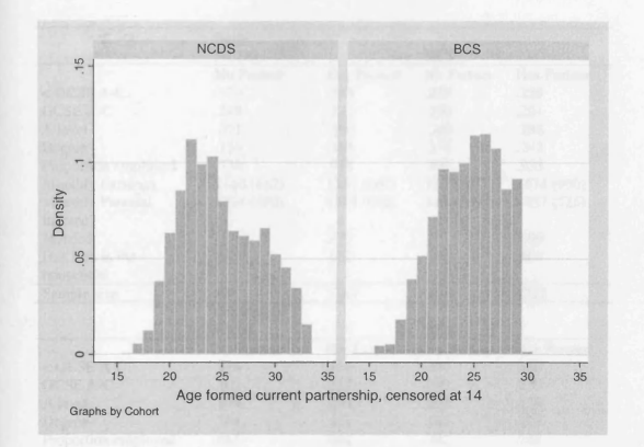

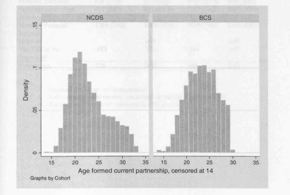
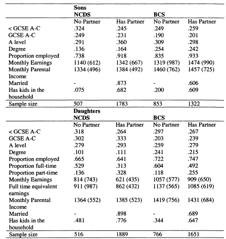


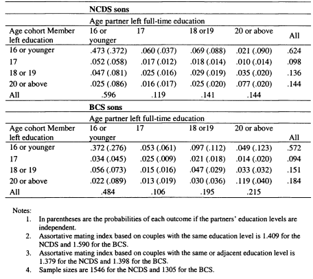

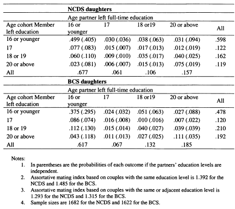
Daughters
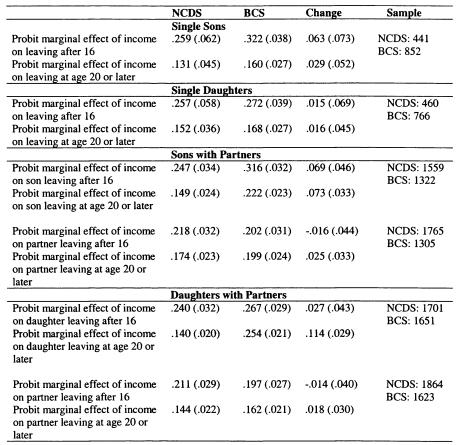


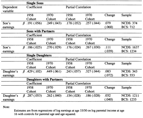
Status

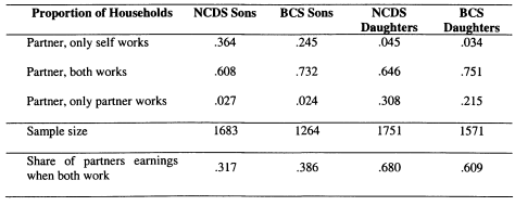

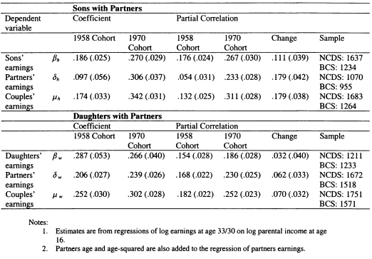

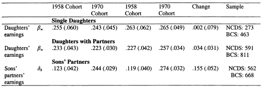
Only

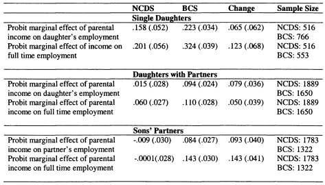
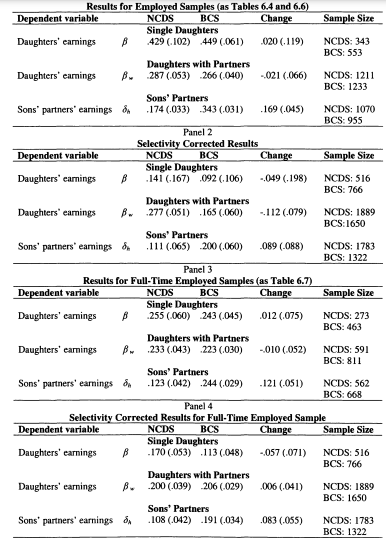


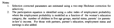
Correcting for Endogenous Participation

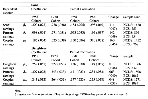
Households, Married Sample
Appendix to Chapter 7: First-stage Regressions for Heckman Corrections Accounting for Selection
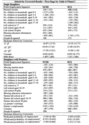


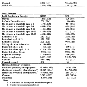
the Selection into Employment
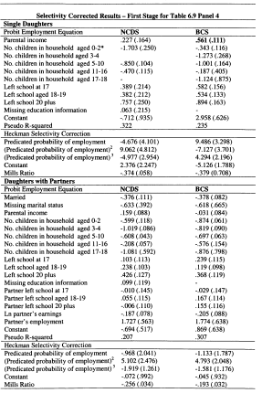


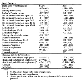
the Selection into Full-Time Employment
Chapter 7: Assortative Mating on Parental Income – Love and Money
7.1. Introduction
Marriage is a crucial institution with the potential to contribute to the persistence of economic and social status across generations and among social groups. As has been shown in the previous chapter for the UK, assortative mating leads individuals to marry people with similar levels of income to their parents, and this contributes to intergenerational income persistence. In this chapter I use unique data to explore intergenerational mobility and assortative mating in Canada. As well as providing a comparative perspective on the UK analysis in Chapter 6, 1 am able to show how couples match on parental income, and I interpret this as a new measure of assortative mating. This is the other side of the interrelationship between household formation and intergenerational mobility. Not only does household formation affect intergenerational mobility but parental characteristics also influence how couples match. Finally I explore how matching on parental income is related to characteristics; including the early dissolution of the union.
In many societies marriage partners have been explicitly chosen by the family to maximize the social position of their children; it is clear that this will result in couples having similar parental incomes55. At first glance, we may think that assortative mating by parental characteristics is not important in a modem society such as Canada where individuals generally choose their own marriage partner and marry for love. However, sociologist William Goode succinctly illustrates why this will not be the case.
Since the marriage population in the US (and increasingly as well as
in other countries) is gradually segregated into pools with similar
social class backgrounds, even a free dating pattern with some
encouragement to fall in love does not threaten the stratification
system. That is, people fall in love with the ‘right’ kind of people56
The Intergenerational Income Data (IID) generated by Statistics Canada (and already used in Chapter 3) provides an ideal opportunity to explore
55 The novels of Jane Austen and her contemporaries confirm the importance of this type of matching in early 19th century England. In traditional Indian society family background as represented by the caste system is important in determining marital eligibility for Hindu families. 56 Goode (1982) page 54
assortative mating on parental income. The dataset was established in order to provide evidence on the relationship between the incomes and earnings of parents and children. The derivation of the data from tax records means that the number of observations is extremely large and so a majority of the women in my sample observed in a partnership in 1998 also have their partners included in the sample. This enables me to match women with their own parents, their partner, and their partner’s parents; a wealth of information not available in any other dataset.
Before showing results for assortative mating by parental income, I examine the extent of intergenerational mobility for sons and daughters in Canada and the contribution of assortative mating to intergenerational mobility. I measure the relationship between parental income and the earnings of sons, daughters and their partners. This follows the analysis explored for the UK in the previous chapter, and emphasises the link between assortative mating and intergenerational mobility. As my sample is based on the cohort of women bom between 1967 and 1970, the results can be compared with those from the 1970 cohort for the UK; this allows a return to the internationally comparative perspective taken in the early chapters of this thesis.
I begin to explore assortative mating explicitly by examining how individuals match on educational levels. As the IID is based on tax data and contains no information on educational attainment I use the Canadian Survey of Labour and Income Dynamics (SLID) to explore this question. I find substantial matching on education, apparently to a similar degree to that which is found for the UK.
In my initial analysis of assortative mating by parental income in Canada I compare the correlation of the incomes of the marriage partners’ parents with that between the earnings of partners themselves. I find that the correlation between the two sets of parents is similar to the association found between the members of the couple.
Measuring assortative mating using parental income correlations is a new venture for Canada. However, assortative mating by educational levels has been considered by Magee, Burbidge and Robb (2000). This paper uses twenty-five years worth of data from the Survey of Consumer Finances to analyse whether couples have become more or less strongly matched on education level over time. The authors find that, on average, the correlation between the education levels of husbands and wives is greater than .6. In addition, it appears to have fallen for young couples over the 1990s.
The connection between the economic status of couples’ parents has been considered for the UK by Ermisch and Francesconi (2002). In this paper (an earlier version of Ermisch, Francesconi and Siedler, 2004, discussed previously) the authors regress Hope-Goldthorpe occupational scores of parents on those of parents-in-law. They find that the elasticity between the occupational indices of parents and parents-in-laws is around .16 while the intergenerational elasticity between parents and children’s occupational indices is around .2. There is evidence, therefore, that matching on parental status is strong.
If the links between parents-in-laws’ incomes is interpreted as a dimension of assortative mating, then we can make a number of predictions about how the extent of assortative matching will vary with the characteristics of couples. I consider the degree to which these predictions are borne out in the Canadian data. As we shall see below, the information available about characteristics is limited in the administrative data used here, but nonetheless the aspects I can observe confirm my expectations. Young people who form unions later appear to be more closely matched on parental income, as do those who are married rather than cohabiting and those brought up in urban compared with rural areas.
In the final section of empirical work I consider whether the strength of matching on parental income influences divorce and separation probabilities. I find that weaker matches between parental incomes are associated with early divorce. This analysis has a precedent in Weiss and Willis (1997) who use data on a cohort of American youth who graduated from high school in 1972 to investigate the determinants of divorce. Weiss and Willis find that individuals with similar education levels are less likely to divorce; this result is also true of common ethnicity and religion.
In the next Section I discuss the theoretical background and empirical approach used in this chapter. Section 7.3 describes the construction of the data set in some detail and reviews the evidence on whether the samples used are representative of the full Canadian cohort. In Section 7.4 I present results on intergenerational mobility for individuals and couples in Canada, while Section 7.5 concentrates on presenting the results for assortative mating. Section 7.6 concludes.
7.2. Theoretical Background and Estimation Issues
Intergenerational Mobility and Assortative Mating
The motivating model used for the first part of this chapter is discussed in Section 2.5 and in Chapter 6, so I simply restate the main implications here. As before, marital sorting results in a positive correlation between the human capital of husbands and wives.
![]()

Combining this representation of marital matching with a simple model of intergenerational mobility generates a number of predictions about the relationships between the education and income of children and their partners and their parents’ incomes.
This model demonstrates how to interpret the intergenerational elasticity for sons and daughters and the intergenerational elasticity for the incomes of partner with respect to parental income. The resulting equations, presented in terms of the daughter’s parental income, ln Y£ mas, are:
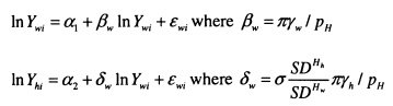

In these equations n is the importance of daughter’s income in her parents’ utility function, yw is the income return to human capital for daughters and pH is the price of a unit of human capital.
There is a strong relationship between flw (the intergenerational elasticity for daughters) and Sw (the intergenerational elasticity between daughter’s partner’s incomes and her parents’ incomes). The similarity between these parameters is clearly closely related to the extent of assortative mating, with larger G meaning that /3w and Sware closer to each other.
In addition, the model provides an interpretation for the relationship between the couple’s total earnings and one partner’s parental income. This is a weighted average of the two parameters J3Wand Sw, with the weighting dependent upon the share contributed by each member of the couple.
![]()

As in Chapter 6 I shall estimate all of the individual intergenerational parameters/3W,S W, /3h, and Sh, as well as the measures of mobility for the couple Hw and juh. These parameters allow me to assess the degree of intergenerational mobility and assortative mating in Canada, and compare it with the results for the UK.
Search Models and Assortative Mating
In Chapter 2 I discussed the predictions about assortative mating that emerge from assignment models of the marriage market. In particular Becker’s (1973, 1974) model predicts a positive relationship between characteristics which are complements in household production. This includes the education levels of partners, unearned income and attractiveness. It is also likely to include parental income as this will be related to characteristics such as education through intergenerational mechanisms (both endowments and investments). In addition, partners may match on parental income if bequests are complements in household production.
A further mechanism will operate if there are direct preferences to match with someone from a similar background. Fernandez et al (2004) explore models where individuals have intergenerational persistence in preferences about women working, meaning that men tend to marry women with the same work status as their mothers. It is possible that other preferences could be similarly transmitted leading to a direct connection between the parental incomes of partners. For all of these reasons we would expect to find positive assortative mating on parental income.
In the original assignment models of the marriage market searching for partners is costless, and the matches that form are stable; leaving no room for divorce or remarriage. In order to place the marriage market in a more realistic framework Burdett and Coles (1997, 1999) and Shimer and Smith (2000) formalise search and matching models of the marriage market to parallel the literature for the labour market. In these models search frictions mean that individuals meet only infrequently. They must decide to either accept each other or wait for the next potential match to come along. Due to these frictions individuals are willing to accept partners who are quite far from the perfect allocation, leading to weaker assortative mating than under a pure assignment model.
Consequently, assortative mating will be weaker for couples whose search is less intensive, perhaps because of higher search costs. In my empirical work I test a number of predictions that stem from this argument. We might expect that cohabiting partners, who might continue to search within cohabitation, may have weaker assortative mating. In addition, longer search will lead to a better match so variation in matching by age at marriage is considered. The cost of search may vary by region, and in particular is likely to be higher in rural areas.
Mortensen (1988) explores the predictions of search models for divorce and remarriage. In this framework there are two reasons for divorce. As noted above, search frictions mean that it is hard to find your ‘perfect’ partner, consequently matches may end if a better alternative is found, even if partners are fully informed about the quality of the match. Divorce is more likely if individuals are far from the optimal allocation. Alternatively divorce may result from uncertainty when individuals only learn about the quality of the match after marriage. In this case the probability of divorce will be positively related to the variance of the unanticipated part of match quality.
Becker, Landes and Michael (1977) and Weiss and Willis (1997) have used similar frameworks to empirically investigate the covariates of divorce. The studies find that couples who are similar on the grounds of religion, education and ethnicity are less likely to divorce. This confirms that couples who are less wellmatched on characteristics (far from the optimal allocation) are more likely to split up. In addition, unexpected events such as infertility or deviations from expected wages are related to higher divorce probabilities, demonstrating the effect of unanticipated match quality.
If the extent of parental income matching acts as a signal of match quality this implies that we might expect that those who are well matched on parental income are less likely to divorce. This hypothesis is possible to test using the IID as partnership histories can be generated for individuals aged up to 30. This interpretation of assortative mating clearly rests on very strong assumption about the way the marriage market operates. It is obvious that unobserved match quality is an extremely important determinant of who marries and divorces, and that this may work to counteract differences in parental background. If we believe that the interpretation of assortative mating as a measure of match quality is too strong, there are alternative interpretations which can be placed on the finding that coming from similar parental backgrounds reduces the probability of union dissolution. For example, it could be that coming from similar family backgrounds lowers the variance of unanticipated shocks as individuals are better informed initially, in line with Mortensen’s (1988) second prediction.57
Estimation Issues
The first results I present here are comparable to those that formed the basis for Chapter 6. I measure the elasticity between the earnings of individuals and their parents’ income and between their partner’s earnings and parental income. Consequently similar empirical problems apply as in the previous chapter. Again I present the full set of results for both genders, meaning that estimates of intergenerational mobility must necessarily be based on current incomes. In Chapter 6 I discussed the biases introduced due to the endogenous selection into work for daughters.
57 Of course, it could also be that there is less tension in marriages when couples are well-matched on parental income.
The income data used in this analysis is based on annual earnings data so there are fewer missing observations than is the case when using weekly data, as more individuals will work at some point during the year. Nevertheless, problems will still result, as fewer of the women in the sample will be working full-time full-year, so that their current income will approximate permanent income less well than it does for men. The main limitation of the IID is that very little addition information on the characteristics of individuals is provided, and the data does not include hours worked. Consequently, it is even more difficult to know how selection mechanisms might affect the results for Canada, and it is not possible to make the adjustments for selection that I used for the UK data. The UK evidence suggests this may cause the intergenerational elasticities to be upward biased when women’s earnings are the dependent variable.
One advantage of the IID data is that information is available for every year. This means I am able to experiment with using three year averages of children’s and partners’ earnings, as a measure of permanent income. While this will be a far from perfect proxy, it will remove some year-to-year fluctuations. However, there is a trade-off. As the most recent data in the IID is from 1998 and the sample is based on those bom from 1967 to 1970, this means that the youngest members of the sample are just 28 when the last earnings data is available. Taking three year averages means using earnings information for some individuals who are as young as 26. Haider and Solon (2004) have demonstrated that measuring earnings at a young age can lead to downward bias. In order to balance these concerns I report both results using the latest data from 1998 and using a more permanent measure of earnings averaged between 1996 and 1998.
Returning to the perennial theme of measurement error in the explanatory variable, the annual data available in the IID should be a better measure of permanent parental income than the weekly data relied upon in some of the other chapters. In addition, this data is averaged over five years from the year when the son or daughter was 14 until the year they turned 18. Both of these aspects of the data should help to reduce measurement error and lower the downward bias in the estimation of intergenerational persistence. Five year averages are used both in the intergenerational estimations and in the equations which estimate the relationships between the incomes of parents-in-law.
7.3 Data and Description of Matching Procedure
Data Description
The data used in this chapter is from the Intergenerational Income Data (IID) a dataset which has already been described and used in Chapter 3. However, the importance of its structure to the estimation carried out in this chapter means that I shall provide a more extensive treatment here. The IID has been constructed from the Canadian Longitudinal Tax Records held by Statistics Canada. The tax records provide information on all income tax returns in Canada between 1979 and 1998. Information on names, addresses and ages included in the data allowed Statistics Canada to match individuals bom between 1963 and 1970 with their parents, this was possible provided both generations filed a tax return while the child was living at home in his or her late teens58.
As the data is based on administrative records its size is considerable: Statistics Canada estimate that the data includes around 70 percent of the relevant age group (Cook and Demnati, 2000). Another advantage of using data based on administrative records is that there is considerably less concern about measurement error and attrition although the unique structure of this data does bring with it additional worries, the main one being that the methods used to match the data may lead to some fundamental sample selection biases, a question I shall return to below.
A second disadvantage of the IID is that there are very few background characteristics available in the data. The information used here is restricted to what is given on the T1 tax return59. Very basic information is available about the individual; age, sex, marital status, spousal Social Insurance Number (SIN), whether the individual filed in French or English and some more demographic information concerning the family in the year the child is matched with their parents. The remaining variables are taken directly from the earnings and income
58 The precise structure of the matching procedure is as follows: individuals are split into three cohorts, those aged 16-19 in 1982, those aged 16-19 in 1984 and those aged 16-19 in 1986. Individuals are matched with parents at any time in the five years surrounding 1982, 1984 and 1986 for each cohort respectively.
59 Other data which has been matched into the IID records is employer information, which is matched through the T4 employer tax form, and geographic information matched in via the postcode on the T 1.
information required on the tax return. In this analysis the main variables used are total employment income (earnings), and “total income” which is the sum of all the income required to be declared on the Tl. “Total income” is earnings, self employment income and asset income (including rents, interest, capital gains and dividends) plus transfers. Which transfers are included varies somewhat by year, for example welfare payments are included in later years, so they are present in the measure of total income for adult children’s income, but not in their parents’.
Individual Intergenerational Sample
Before considering assortative mating I present estimates of intergenerational mobility by gender and partnership status. For these models I use samples constructed on the same basis as those used to explore intergenerational mobility for Canadian sons in Chapter 3. These samples include all sons and daughters bom between 1967 and 1970. I extract two measures of income for the two generations: annual earnings and annual total income. Parental income is defined as the average of income when the child was 14 to 18.1 exclude income/earnings reports of less than $ 160 for parents and $2 for the adult children.
Matching Spouses
There are two features of the data which allow the matching of couples with both sets of parents. First, we have information on the SEN of spouses and cohabitees. Second, the near universality of the data means that many of the spouses/ cohabitees of those included in the data will have intergenerational records. A limitation is that SINs are not obtained for all cohabitees. Married individuals are always asked to state their spouse’s SIN on their tax return but individuals were not asked for their cohabitee’s SEN until after 1992. Also, the definition of cohabitation is more restrictive than in other surveys. Partners are defined as cohabitees if they are the natural or adoptive parent of the individual’s children, if they have lived together continuously for a year or had lived together for a year in
60 There is some bunching at very low levels of income and earnings in all years. It is important to take account of these observations as they are almost certainly a consequence of mis-measurement. I have experimented with a variety of methods and the precise approach used appears to make little difference to the results obtained.
the past. This means that the matches found will miss the shortest cohabitations, a limitation which has advantages and disadvantages. The sample will not be representative of all couples, but results will not be distorted by the inclusion of very temporary cohabitations.
In order to construct the spousal sample I focus on daughters bom between 1967 and 1970. I am then able to search for the ‘spouses’ for these women from the entire IID sample of men bom between 1963 and 1970, allowing for the fact that women often marry men somewhat older than themselves. I shall comment more on this feature of the match when I discuss how representative the data are.
1998 Spouse Sample
The first sample I use is couples who are married/cohabiting in 1998. The first stage is to match daughters who filed for tax in 1998 with their spouse’s tax return for 1998. Fortunately, 98 percent of those who declare themselves to be married or cohabiting in 1998 include their spousal SIN on their tax return. As shown in Table 7.1 there are 511,636 women bom between 1967 and 1970 in the dataset, 294,251 of whom file tax returns in 1998 and state that they are married or cohabiting. 179,341 couples are matched on the basis of their 1998 returns, 60 percent of all the women who report having partners in 1998. There may be a concern that by matching couples on the basis that both file in 1998 will introduce a selection bias. This would be a particular difficulty if women filed less than men because of weak labour market attachment. The evidence suggests this is less of a problem than we might imagine with 7 percent of males in the IID not filing in 1998 compared with 11 percent of females. In order not to miss individuals who do not file in 1998 I adopt a second stage to the match based on all years on data. This adds an additional 5000 couples to the sample.
Divorce and Separation Sample
The first sample of couples I create is of all surviving partnerships in 1998. However, this will not enable me to explore the dissolution of partnerships. To do this I create a separate sample which matches couples in the year that the partnership is first observed in the HD, i.e. the first year that a spousal SIN is listed. This approach means that I am able to track all the partnerships listed by an individual, and match partners when they are included in the IID61. The obvious difficulty is that I am only able to match partnerships when the sample individuals are young, up to 31 at the oldest, so only early partnerships and dissolutions are included.
In my 1998 sample of couples I match both those who are legally married and those who are cohabiting. As the marital status “cohabiting” was not included on the tax return until 1992 this is not possible for the full relationship history, so before 1992 cohabiting partners are necessarily excluded. In my empirical work I deal with this is two ways. One approach is to use both types of partnerships but exclude any first observed before 1992, the second is to consider only those partnerships which resulted in marriage, and take the starting point from the year the individual first reported herself as married.
Are the IID Samples Representative?
Owing to the sample selections inherent in the intergenerational matching procedure employed in the construction of the dataset, it is important to establish that the samples obtained from the IID are representative of the population of interest. Individuals are only included in the sample if at least one parent files for tax in a year that the child is living at home and also files for tax. Compulsory tax filing in Canada means that children will file even if they are only undertaking part-time or holiday work while in education, but concerns remain. Families who are excluded from the IID may come from the lower part of the income distribution (parents have no labour market attachment, children are unemployed or work in the underground economy) or the upper end (children are in education and do not work at all). As explained by Oreopoulos (2003) the likelihood of the second outcome is reduced by the ability of those in full time education to obtain tax credits and deductions by filing.
Oreopoulos (2003) and Corak and Heisz (1999) both explore the representativeness of the IID. Oreopoulos finds that those who are missing from
61 Further work is needed to understand how this sample may be affected by the sample selection issues inherent in the IID.
the IID tend to have somewhat worse socio-economic characteristics than the average while Corak and Heisz find that the IID is somewhat better than survey data at picking up observations at the very extremes of the distribution. In addition Corak and Heisz estimate a sample selection correction model for those who are matched to fathers and find that the correction makes essentially no difference to their estimates of intergenerational mobility.
Tables 7.2 and 7.3 present my own investigation of these issues. First, I compare the key characteristics of all women in the IID bom 1967 – 1970 who are single in 1998 with those with partners (according to the tax definition), and most importantly, those who I can match with partners in the IID. This will demonstrate whether the process of spousal matching employed introduces further biases to the IID sample. In Table 7.3 I show the characteristics of women from the same cohort observed in the 1998 SLID sample, again by partnership status. This demonstrates the features of the IID sample in comparison with a nationally representative, if small, sample.
My comparison of single women in the HD with those with partners (Table 7.2) indicates that women with partners are slightly less likely to file positive earnings, and have somewhat lower earnings and parental income (this likely to be a result of a negative relationship between parental income and the age at which women form partnerships). More interesting is the comparison of all women with partners with women matched with their partners in the IID. There is evidence that daughters and their parents who are matched are slightly better off. Their own earnings are on average $400 higher than all women with partners, and their parents’ incomes are $1000 greater. This is not surprising. If we believe that the IID in general has a slight bias to those with higher incomes then it is no surprise that restricting the sample to those with partners in the IID will strengthen this bias.
The evidence that my sample may be skewed towards the better off is confirmed by the figures in Table 7.3, which shows the characteristics of women bom between 1967 and 1970 in the 1998 SLID. For both single women and those with partners average annual earnings in 1992 dollars are about $l,500-$2,000 higher for the IID samples than they are in the comparable samples in the SLID62.
The SLED data shows the consequence of the strict definition of a cohabiting couple in the tax data. The proportion of the sample that is recorded as having partners is larger in the SLID than in the IID sample, and a lower proportion of women in partnerships is married rather than cohabiting in the SLED compared with the IED63.
The SLED data can also be used to provide information on partner’s age for the women in this cohort. This is important as the structure of the IID means it is only possible to match up those spouses bom between 1963 and 1970. Of women bom between 1967 and 1970 with partners in 1998, 72 percent marry men bom between 1963 and 1970. Assuming that the age distribution of partners is the same in the IED as in the SLID (a strong assumption as the definition of cohabitation used to construct the samples is not comparable) and given that we know that the HD covers 70 percent of the cohort, I would expect to match just over 50 percent of women with their partners. In fact, I match 63 percent. This suggests either that women in the IID are more likely to be cohabiting with or married to men bom between 1963 and 1970 than those in the SLID, or that the coverage rate for these partners is higher than 70 percent. A higher than average coverage rate for the partners of women in the sample suggests that the probability of women and their partners being in the IID is positively correlated.
7.4. Results on Intergenerational Mobility
Intergenerational Mobility for Sons and Daughters in Canada
Table 7.4 shows the intergenerational mobility of sons and daughters in Canada by partnership status. This provides a background to the discussion of the contribution of assortative mating to intergenerational persistence, and allows a
62 There is also some evidence of a different regional composition in the two samples. The IID has a lower proportion of the sample than the SLID in Ontario and British Columbia. A lower proportion in the IID in Montreal and Vancouver is found in Corak and Heiss and is attributed to the exclusion of recent immigrants from the IID.
63 As access to the SLID is restricted, at this stage it is not possible to construct a sample in which cohabitation is defined in a way more similar to the tax data. This will be attempted in subsequent analysis.
comparison to be made between Canada and the results for the UK shown in the previous chapter.
All the results indicate comparatively high mobility in Canada, as shown in Chapter 3 and in line with Corak and Heisz (1999). Estimates in Table 3.3 when two year averages of parental income are used as the explanatory variable showed that the intergenerational correlation in the US and UK is around .3. The estimates shown for sons and daughters in Table 7.4 are closer to .15. This is despite the fact that the five-year averages available in the Canadian data would encourage us to think the Canadian estimates are less attenuated by measurement error. Parameters are higher when average measures for 1996-1998 are used, showing that even for young people averaging earnings over several years reduces downward bias.
Here we are interested in how estimates compare for sons and daughters and for those who are single compared with those in couples. The elasticities suggest that intergenerational persistence in Canada is approximately equal for sons and daughters; however the correlations show that persistence for men is stronger than for women. Although the difference in the correlations is small the large sample size means that it is statistically significant for those in couples. Results based on the average dependent variable show that the intergenerational correlation for sons with partners is .185 (.002) compared with .168 (.002) for daughters with partners.
In all but one case, Table 7.4 reveals that intergenerational mobility is weaker for those in couples than for single individuals, for both men and women. For women this may be because lower annual hours among married women are correlated with low parental income. Another explanation is that the difference between single and partnered individuals is associated with age within the cohort: single individuals are likely to be younger and this is associated with lower estimates of earnings persistence. This will be investigated in further work.
Comparing these results with those for the UK from Chapter 6 paints a mixed picture. As already noted, intergenerational persistence is low in Canada compared to results for a similar cohort in the UK64. However, one common factor which emerges from the analysis of intergenerational mobility in the UK and Canada is that the intergenerational mobility of own earnings is greater for daughters in couples. As in the UK, this motivates the analysis of the role of sonsin-law in contributing to persistence in Canada.
In this section I have explored the relationship between the earnings of adult children and parental income. The tax data available means that there are a number of alternative income measures which could be used as both the dependent and explanatory variable. For reasons of space I do not show the full range of results here. However, one particularly striking result is that in every case but one (daughters in couples) the elasticity and correlation between the child’s total income and total parental income are stronger than those between the child’s earnings and parental income. In the total income specifications the intergenerational correlation approaches .2. This implies that parental endowments and investments affect welfare in ways additional to labour market performance.
Intergenerational Mobility and Assortative Mating
The next step in the analysis is to examine how assortative mating and individual intergenerational mobility interact to drive intergenerational persistence between families. In Table 7.5 I use the matched sample of those in couples in 1998 to show results for individual intergenerational mobility, alongside the elasticity between partners’ earnings and parents’ income and between parental income and the total earnings of the couple. For the UK, results for the 1970 cohort (shown in Table 6.6) demonstrate that partners’ incomes were strongly related to individuals’ parental income and that this was true for both sons and daughters. This contributes to a picture of strong intergenerational persistence over total family earnings.
The first two panels of Table 7.5 show results where the daughter’s parental income is used as the explanatory variable. As the IID data also provides
64 It is notable that results for Canadian sons are of a similar magnitude to those for the earlier UK 1958 cohort (NCDS) in Tables 4.2 and 6.4.
information on her partner’s parental income the lower panels report estimates for the same sample where her partner’s parental income is used as the explanatory variable. Such a comparison was not possible using the UK data.
Turning first to the results for individual persistence, it is reassuring that these are very similar to those obtained for all sons and daughters in couples in Table 7.4. Even though the descriptive statistics in Table 7.2 showed that women who are matched with their partners tend to be slightly better off, this suggests that the rest of the results presented for matched couples should not be biased by selection into this sample.
The easiest way to evaluate the contribution of assortative mating to intergenerational persistence is to see how /? (individual persistence) and // (the persistence for the couple as a whole) compare, if /z > ft this indicates that adding partner’s earnings to the story is increasing measured intergenerational mobility. In all cases the partial correlation measure of /z exceeds/?. This is more pronounced for women than men.
The fact that assortative mating makes a more important contribution to intergenerational persistence for women is in line with the traditional view that marriage is important in securing the social position of women, but less important for men. In this data this comes about for two reasons. First, the correlations between daughters’ earnings and parental income and their partners’ earnings and parental income are almost equal for daughters; whereas for sons they are more dissimilar. Secondly, partners contribute a larger share of the household income for daughters, around 37 percent of household income, the importance of this os shown by the decomposition of couple’s earnings persistence, /z = (1 – s)fl + s S .
Results for the UK showed that for the second cohort, at least, partners’ earnings play an important role in generating intergenerational persistence for both men and women, although the importance of partners’ earnings was stronger for daughters. These conclusions are replicated for the analysis of a similar cohort of Canadians.
7.5 Results on Assortative Mating
Assortative Mating by Education
In this section I consider assortative mating directly. As the IID has little information about personal characteristics, I cannot compare my new approach to measuring matching based on parental income with a more standard model of matching based on education. I therefore begin by using the SLID to investigate matching on education level. Again, this replicates one of the approaches taken to the analysis of the British cohort data in Chapter 6.
In Table 7.6 I demonstrate the distribution of educational attainment for the sample drawn from the SLID. This sample is based on 1998 data and includes all couples where the ‘wife’ is aged 25 to 40 at the time of the survey. The tabulation of education levels reveals a strong concentration of the sample at the ‘further education’ level; almost half of both the male and female partners are in this category. It also demonstrates that women tend to be slightly more educated than men in this sample, being less likely to drop out of school, and somewhat more likely to obtain a degree.
Table 7.7 shows the relationship between the education levels of couples in this sample. The first number displayed in the upper panel is the proportion of couples with each combination of education levels. In parentheses I show the proportion expected in each cell if education levels are independent within couples. This compares the actual distribution with the counterfactual distribution if there were random matching. The lower panel makes this comparison more explicit by showing the ratio of the two (in other words, how much more likely the combination is for couples than would be expected).
As in the UK, there is evidence of assortative mating by education levels. In all cases the number on the leading diagonal of the lower panel is greater than one, indicating that individuals are more likely to marry those with similar education levels. Also, cells that are further away from the leading diagonal have smaller ratios. For example, combining the independent probabilities that men and women drop out means that 2 percent of couples would be formed of men and women who are both drop outs. In fact 5 percent of couples have this outcome, meaning it is more than two and-a-half times more likely than we would expect. Similarly, 3 percent of couples would be expected to consist of a ‘drop-out’ husband and a graduate wife, less than 1 percent of actual couples have this combination.
In order to aggregate the results shown in Table 7.7 I calculate the proportion of couples which share the same education level and compare this with the proportion expected to do so if education levels were independent. I find that 49 percent of individuals match with someone in the same education group, while 32 percent would be expected to do so. Taking the ratio of these gives 1.514, the aggregate measure of assortative mating on education. Expanding the definition of matching to also include those who match with a partner in the adjacent education group reduces this measure to 1.174. While the distribution of education levels is clearly very different in the UK, it is still possible to compare these aggregate measures. The numbers derived in Tables 6.2A and B for the British Cohort Study range from 1.5 to 1.6 for those in the same category and 1.3 to 1.4 for those marrying someone in the same or adjacent group. The conclusion of this comparison is that the extent of assortative mating on education in the UK and Canada appears to be similar.
Assortative Mating by Earnings, Income and Family Background
Table 7.8 reports elasticities and correlations between alternative measures of economic status for couples in the IID65. Three sets of results are presented, those for earnings and incomes for the couple in 1998, results for these measures averaged over 1996-1998, and results for five year averages of parents’ and parents-in-laws’ earnings and income. The elasticities and partial correlations provide average measures of assortative mating, meaning that it is straightforward to compare the extent of assortative mating by different variables.
In Becker’s analysis of assortative mating, he predicts that individuals will match negatively on wages and positively on unearned income, because wages are substitutes in the production of market goods. However, negative matching on wages will only be found if all of the correlation between wages and non-market productivities can be stripped out, as these will be complements in producing
65 Descriptive statistics for this sample are shown in the appendix.
household goods. We would expect to find an unconditional positive relationship between the wages of a couple. The first model in Table 7.8 uses annual earnings rather than wages, these include the impact of joint household labour supply decisions, complicating the story even further.
The strongest correlation observed between partners’ income or earnings is for the three year average of earnings: the correlation in this measure between ‘husbands’ and ‘wives’ is .16. Assortative mating is stronger on own earnings than on own income. However, the correlations between the market and total income of partners are difficult to interpret as in some cases joint assets may be assigned to one partner on the tax return in order to attain the optimal tax treatment. As expected, the use of averaged measures of incomes raises the observed correlation between couples66.
The lower panel of the Table reports the elasticities and partial correlations of daughter’s parental income with respect to her partner’s parental income. It is clear that the extent of matching on parental income is very similar to the extent of matching on earnings within a couple. The correlation between earnings with the couple is .16 while the correlation between parental incomes is .19. Results for parental income are stronger than they are for parents’ earnings, illustrating that total resources drive matching on parental characteristics.
Ermisch and Francesconi (2002) explore the correlation in occupational indices of parents using data from the UK, and find it to be around .16, slightly lower than the correlation in occupational status between parents and their children in the same sample. For Canada, the correlation between the incomes of parents-in-law is .19. This is stronger than the relationship between parental income and children’s earnings but very similar to the correlation in total incomes between generations, which I find to be close to .2. This implies that, in Canada, the degree of horizontal income persistence (between parents-in-law) is similar to the degree in vertical income persistence (between parents and children).
66 The sample sizes are smaller for the second panel as not all couples were couples in all years, but differing sample sizes do not explain the difference between the single year and averaged results.
Variations in Assortative Mating
Table 7.9 shows how assortative mating on parental income varies with some of the characteristics observed in the IID. The motivation behind this is to test if assortative mating on parental income is low in cases where we would expect search to be less intensive. I therefore test the relationship between assortative mating and the following variables: cohabitation, age at the start of the relationship and urban/rural residence. The Table shows the coefficient on daughters’ partners’ parental income in a regression of her parent’s income, and the coefficient on this variable when interacted with the characteristic of interest. I do not show partial correlations to account for different variances, as this adjustment has little effect for the parents-in-law results.
Cohabitation in Canada, as in many other developed countries, has risen rapidly over recent years. Wu (2000) provides an extremely thorough investigation of this change, the possible reasons behind it and its implications. Between 1981 and 1996 the number of families that included an unmarried couple rose from 1 in 17 to 1 in 7 (Wu 2000: pi). As shown in Table 7.2, in my sample 15 percent of the matched couples are in cohabiting unions rather than marriages. How can these cohabiting unions be interpreted? Clearly they do not have the legal standing of marriages and we may therefore expect they will, on average, be entered into more casually. In addition, cohabitations are frequently short: half end within three years. However, the majority of cohabitations that end within three years become marriages, this implies that cohabitations (particularly for the young) can be thought of as trial marriages. Wu (2000: p3) puts this explicitly in terms of assortative matching.
…cohabitation can be seen to perform the function of a ‘trial
marriage’, weeding out the ‘bad matches’ from the assortative
matching process and keeping the good ones.
With this hypothesis in mind we may expect cohabiting unions to have lower associations between parents-in-laws incomes than marriages. The first result shown in Table 7.9 shows that this is, indeed, the case: while the average elasticity between parents-in-law’s incomes is .183 the elasticity for those in cohabiting unions is .03 lower than for those who are married. This result has indirect support from studies examining matching for couples in the US 1990 census. Both Blackwell and Lichter (2000) and Jepsen and Jepsen (2002) find that correlations between the education and race of partners is lower among cohabiting couples.67
The second hypothesis I test is whether the parents-in-law elasticity varies with the age at which the partnership is formed. The educational homogamy literature (Mare, 1991, Chan and Haplin, 2003, and discussed more fully in Chapter 6) has stressed the importance of the number of years between age at marriage and age left education as determining the closeness with which couples match on educational level. If marriages form soon after school leaving age they are more likely to be with former class-mates, implying a negative relationship between the closeness of matching and age at marriage. Other studies have stressed that a later age at marriage means that individuals have searched more. Weiss and Willis (1997) show that a later age at first marriage is associated with a lower probability of divorce.
The second result presented in Table 7.9 shows the interaction between the age the relationship began and the parents-in-law elasticity. This interaction is small, but significant; for every year that individuals wait before beginning a partnership the association between their parental incomes is increased by .002, so if individuals wait five years the elasticity is increased by .01. This provides some support for the Weiss and Willis finding that longer search leads to a ‘better’ match.
Another dimension on which theory has implications is population density. If assortative mating is interpreted as the outcome of a search process we would imagine that young people in rural areas will find it more difficult to match. Once again this hypothesis finds backing in the IID data; the elasticity of daughter’s parental income with respect to her partner’s parental income is .018 lower for daughters who grew up in rural areas. This result is robust to controlling for province and for province interacted with partner’s parental income.
We might also be interested in how mobility varies by region, particularly for Quebec, as it is culturally the most different of the provinces. A feature of
67 Of course this result has other possible interpretations which lie outside a search framework. It could be that individuals from similar family backgrounds find more family support for their union and therefore are encouraged to marry more often/earlier.
family formation in Quebec is extremely high rates of cohabitation and low rates of marriage in the province. Wu (2000: 47) shows that in 1996 almost 25 percent of unions in Quebec were cohabitations compared with around 10 percent in the rest of Canada. I find that Quebec is fairly typical in the extent of assortative mating on parental income. To explore this further, I have checked if there are any differences by the official language used on the tax return. There is slight evidence that those who file in French have a lower match on parental income. However, this small effect is driven by comparing Quebec with the rest of Canada, and there is no effect for francophones outside Quebec.
The results presented in Table 7.9 show that the extent of matching on parental income varies along some dimensions of daughters’ and parents’ characteristics. In terms of cohabitation, age at union and rural residence these variations are consistent with a search framework of the marriage market where the extent of parental income matching provides a measure of assortative mating.
Divorce and Assortative Mating
If the extent of parental income matching provides a measure of match quality we should expect that those couples who are more closely matched have more stable relationships and are less prone to divorce and separation. This final empirical section explores this question using partnership histories for daughters. As described in the data section this enables us to have information on all partners who are also included in the HD since 1992 (and their parental incomes) and all marital partners who are within the IID. By using information about spousal SIN and marital status I am able to observe if the daughter is still with each partner by 1998.
Table 7.10 provides descriptive statistics on partnership formation and disillusion for both samples. The lower panel of Table 7.10 presents the descriptive statistics for all marriages from 1986 onwards. Few marriages begin in the early years of the survey and this rises steadily through the data, peaking in 1993 when 12.4 percent of marriages begin. It is clear that early marriage is an important determinant of whether a partnership lasts; annualized divorce and separation rates are higher for those who marry early.
In the lower panel descriptive statistics are considered for the post-1992 sample. These reveal some difficulties of definition. The divorce rates indicate that partnerships formed more recently are much more likely to end in divorce or separation. Of partnerships formed in 1992 4 percent of couples are divorced by 1998 and 12 percent are separated, this is .07 and 2 percent per year respectively. Of those formed in 1997 8 percent are divorced by 1998 and 21 percent separated. While we might anticipate that cohabitations are short and frequently end in separation, it seems unlikely that the result for divorces is correct, particularly as it is not found for the sample of marriages. My explanation is that people who are actually cohabiting are reporting themselves as divorced with reference to an earlier relationship68. This problem means that the results for cohabiting couples should be treated with more caution than those for the sample of marriages.
The relationship between divorce, separation and parental income matching is explored in Tables 7.11 and 7.12. Table 7.11 considers all marriages. In the first column of the Table I control only for the ages of the daughter, her partner and both sets of parents. I find that those partnerships which end in divorce had a substantially lower correlation between the parental incomes of the woman and her partner, the coefficient on the interaction is -.056 (.008) and there is also a negative relationship between separation and matching on parental income, at -.017 (.007) in the last column. In the remaining columns I attempt to control for explanatory factors which may be related to both partnership dissolution and the extent of assortative mating. Adding controls for province and the year in which the couple began cohabiting does reduce the interaction effects but they remains strong at -.049 (.010) for divorce and -.17 (.007) for separation.
Table 7.12 considers the sample that began their partnerships in 1992 or later, as before, and in addition, whether the couple are legally married or not. Once again there is a strong negative interaction effect between divorce and parental income, while there is no difference between the extent of matching for couples who separate compared with other couples. As noted above, these results should be treated with caution, but the fact that they are similar to the more solid data for marriage is reassuring.
68 An alternative way to consider the end of cohabitations would be to look at changes in the reported spousal SIN.
Evidence for Canada strongly suggests that couples who are more closely matched on parental income are less likely to divorce or separate. It is possible that this result is driven by particularly high divorce probabilities for couples from very different backgrounds. To explore this, I divide parental incomes into quintile for both partners and compute divorce probabilities by parental income pairs. I do this by comparing the probability of divorce for a couple if divorce was independent of the interaction of parental income and compare this with the actually divorce probability for couples with that combination of parental income quintiles. As shown in the appendix tables A.7.2 and A.7.3 I find no clear pattern that the relationship between parental income matching and divorce is non-linear.
7.6 Conclusion
In this chapter and the one which preceded it I have attempted to evaluate the contribution of assortative mating to intergenerational correlations in household earnings. Analyses that take account of the role of partners’ income are rare in the intergenerational income mobility literature and I am able to add results from two more countries, Canada and the UK, to build upon the recent analysis for the US conducted by Solon and Chadwick (2002). As in Solon and Chadwick, assortative mating is shown to add an important dimension. The partial correlations between the couple’s earnings and parental income are higher in both cases than the correlations between individual earnings and parental income. In both cases recent data shows this effect to be more important for the intergenerational persistence of women, but it is also important for men, an aspect overlooked in previous investigations.
Due to the unique data available for Canada I am able to explore the level of matching on parental income within couples. This provides evidence on a new dimension through which parents and children are linked. I show that matching on parental income is substantial; indeed the correlation between parents-in-laws’ incomes is very similar to the correlation found in income for parents and their offspring in Canada.
This finding is interesting in itself; however, owing to the correlation of parental income with many other characteristics of the two partners, I interpret the match on parental income as a general purpose measure of assortative mating. Consequently, I test a number of hypotheses which would emerge from a searchtheoretic framework. In all cases the results justify my approach; the extent of assortative mating rises with the length of search (age at which the partnership is formed) and the thickness of the market (urban v rural area) and weaker assortative mating is associated with a higher probability of the match dissolving.
This preliminary exploration of parental matching has opened up a number of avenues for future research. It is clear that some of my analysis requires development to firm up the mechanisms through which the match on parental income operates. It is also true that the theoretical link between divorce and the extent of assortative mating on parental income should be formalised. Nonetheless, the fact that my empirical results are in line with the intuitive predictions of search models encourages me to pursue this line of investigation. In addition, it would be extremely interesting to explore these issues using data which contained more information about the characteristics of parents and children; in this regard Nordic register data has interesting possibilities69.
69 R0ed and Raaum (2003) provide an interesting discussion of the development and use of these data in Norway.

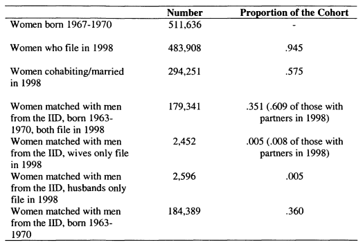
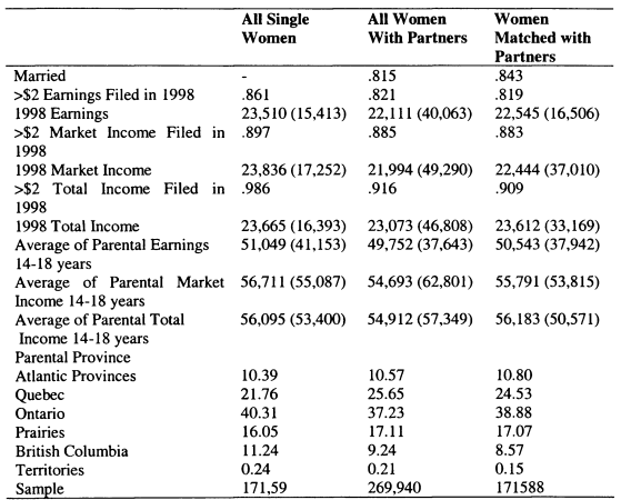


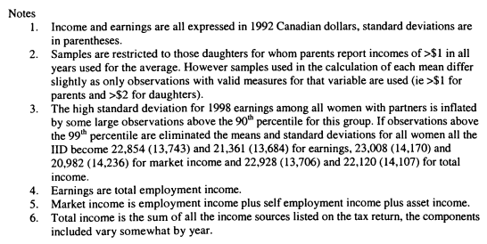
With All Women in the IID

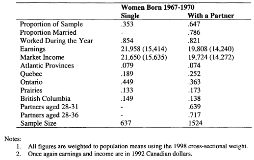

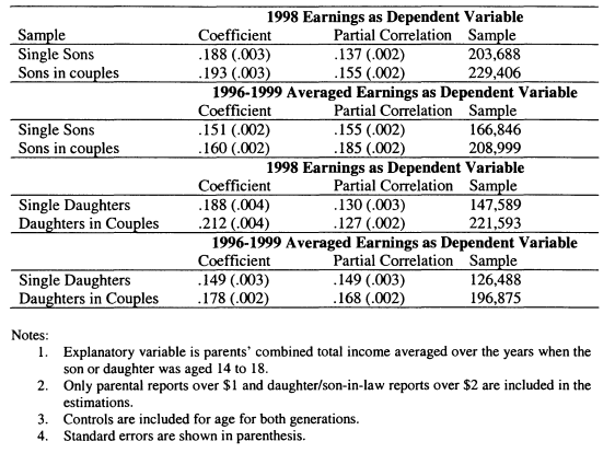
and Partnership Status

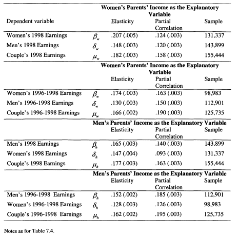

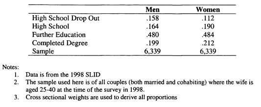

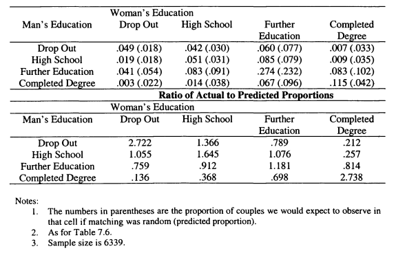

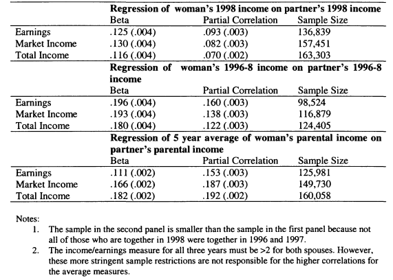

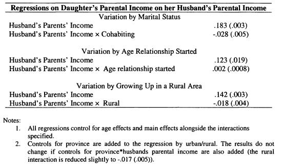

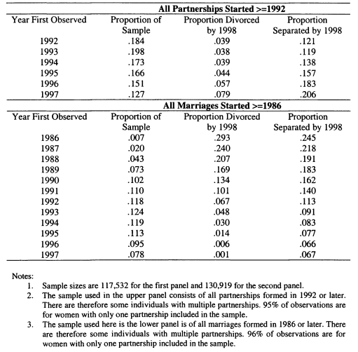

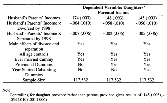
Partnerships

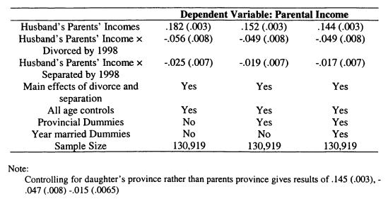
Appendix to Chapter 7: Further Descriptive Statistics

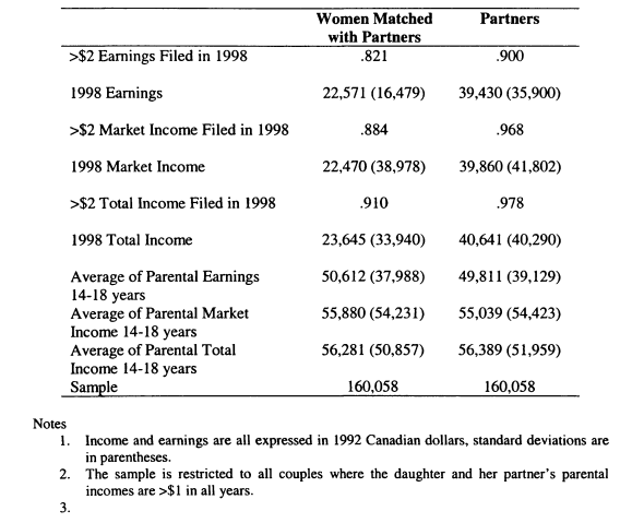

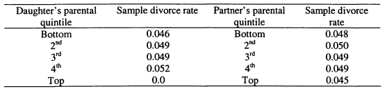

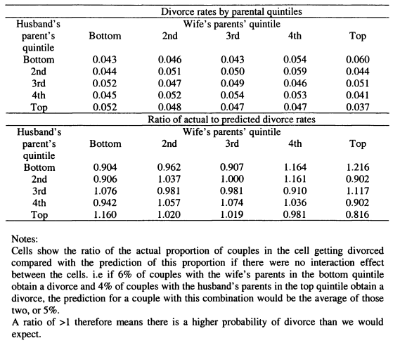
Chapter 8: Conclusions
The New Labour Governments from 1997 onwards have put social justice as one of the central tenets of their political philosophy. As with many political concepts this is to a certain extent a catch-all – used to describe the merits of many policies. However, one aspect which is returned to repeatedly is the value of making sure that all children have the chance to fulfil their potential; a concept clearly connected to intergenerational income mobility. In a recent speech setting out New Labour’s vision for a third term, Alan Milbum emphasised a commitment to equality of opportunity.
There is a glass ceiling on opportunity in this country. In our first two terms we
have raised it. In our third term we have to break it. I believe we can do more in
a third term to create an inclusive economy and the opportunity society than we
were able to in our first two.70
With social mobility a policy goal du jour at the start of the 2005 general election campaign, this thesis provides a particularly timely discussion of intergenerational income mobility in the UK. In addition, I place my discussions firmly in an internationally comparative framework, and conduct new analysis of how intergenerational relationships are affected by (and affect) household formation.
The first question I address is how the level of intergenerational mobility in the UK compares in an international framework; comparing findings on sons from UK data with methodologically equivalent estimations for the US, West Germany and Canada. In general, this analysis supports the picture painted by comparing the evidence from single country studies. The US and UK appear to have fairly low mobility, while mobility in West Germany is moderate and Canada appears to be the most mobile of these countries.
This investigation does reveal a number of new points, however. First, there are some clear differences in the estimations depending on whether parental income or father’s earnings is used as the dependent variable, which suggest opportunities for further research. Also I consider the contribution made by education to intergenerational persistence. It appears that the low mobility in the US is related to
70 Alan Milbum MP’s speech to the Fabian Society on Sunday January 16 2005. Milbum is currently Chancellor of the Duchy o f Lancaster and in charge of the Government’s election strategy.
the high earnings returns to education, while both in the UK and the US the strong relationship between parental income and educational attainment is notable.
My cross-country analysis also teaches an important lesson about what we do not know. The standard errors in my analysis are quite large for all countries apart from Canada. This means that the only strong conclusion which can be taken from this strictly comparable investigation is that mobility in Canada is greater than in the US and UK. Corak (2004) provides a recent survey of the literature on cross-country comparisons, which attempts to make adjustments to the estimates to account for noncomparability in the estimation approaches. Corak’s approach leads to qualitatively similar results to the ones I find, and also allows the examination of more countries than I consider. However, the assumptions made to ensure comparability are likely to add to the uncertainties caused by sampling variation, and no standard errors are provided for the preferred estimates. An advantage of my approach is that the uncertainties caused by sampling variation are made explicit, even if the results initially appear to be less concrete.
The second empirical chapter of my thesis also approaches intergenerational mobility from a comparative perspective, but this time comparing changes over time for the UK and US. In Chapter 2 I demonstrated that there have previously been few studies addressing the change in mobility over time. The studies on income mobility that have been carried out to date for Norway, Finland and Canada have pointed either towards no change in mobility or an increase. In sharp contrast, the data reveals a very clear picture of falling mobility for the UK; when comparing sons bom in 1958 with those bom in 1970.1 also revisit the data for the US where previous studies have pointed towards an increase in mobility. I find no evidence of a change when comparing cohorts bom between 1949 and 1970 and while there is evidence of a small decline in persistence followed by a steep rise in later cohorts, there is insufficient information to be confident that these are the result of anything but sampling variation. This indicates that the findings of a rise in mobility from previous studies do not appear to be robust given the data available. There is certainly no evidence of a strong and significant fall in intergenerational mobility in the US to mirror the one found for the UK.
Motivated by the finding of a large increase in intergenerational persistence for British men, I examine the role of education in generating the level and change in intergenerational persistence for the UK. My findings are striking. Despite the expansion of the number of students undertaking higher qualifications, the distribution of these opportunities has been skewed towards students from higher income backgrounds. This partially explains the reduction in intergenerational mobility found for the UK.
As part of my exploration of the relationship between education and parental income I attempt to provide some evaluation of the mechanisms that lie behind intergenerational persistence. As reviewed in Chapter 2, the classic models of intergenerational mobility highlight inherited characteristics and investments as the twin mechanisms through which income is correlated across generations. If the investment mechanism is important we will find a causal relationship between parental income and educational attainment. Finding that income matters in and of itself has two important implications; first prices and returns will influence intergenerational mobility as parents are making decisions about investments. Second, government policies on redistribution will influence the outcomes of poorer children. I find that there are causal impacts from parental income to educational attainment; but these are small compared to the differences in education observed between those from rich and poor backgrounds. This appears to support the Government’s emphasis on tackling educational inequalities directly rather than through redistribution.
The first part of my thesis followed the majority of the literature on intergenerational mobility in stressing the relationship between individual earnings and parental income. But consumption (and thereby utility) depends upon both the individual’s own income and his or her partner’s income. Only very few studies have considered the role of partners’ earnings in generating intergenerational persistence. In those that have been carried out (e.g. Chadwick and Solon, 2002, Atkinson et al, 1983 and Lam and Schoeni, 1994) the focus has been very strongly on the relationship between women’s fathers’ earnings and her husband’s earnings, largely ignoring the relationship between women’s earnings and both their own parental income and the parental income of their partner. In the final chapters of my thesis I widen my consideration of mobility to take into account the contribution to intergenerational mobility made by partners, and I look symmetrically at the role of sons, daughters, husbands and wives.
For the UK, I revisit the findings on changes in intergenerational mobility for sons and add an analysis for daughters to this picture. I find that the decrease in intergenerational mobility is not as strong for daughters as it is for sons. When I add partners’ earnings and examine the persistence in family earnings between the two generations, I find that the change in mobility for sons is even stronger than first thought. It is clear that for the later cohort the earnings of sons’ partners have become as closely related to parental income as they are for daughters’ partners, a particularly striking finding given that the literature had focused entirely on the relationship between daughters’ partners and their parents up to this point. This ‘daughter-in-law persistence’ adds substantially to the extent of intergenerational persistence for sons.
For Canada, I am able to build upon this further. Using a very large dataset based on tax returns I am able to, for the first time, link the incomes of both sets of parents for many couples. In this dataset, as for the UK, I find strong links between partner’s earnings and parental income for both men and women. Once again assortative mating makes a strong contribution to intergenerational persistence. A new dimension to the intergenerational relationship is explored by considering the way that couples match on parental income. This shows that not only does choice of partner influence the correlation between children’s and parents’ incomes, but that parental income has a bearing on how couples match.
I find that the correlation between parents-in-laws incomes is .2; approximately the same as the intergenerational income correlation in Canada. Treating this correlation as a new measure of assortative mating, I am able to make a number of predictions about the way in which the extent of assortative mating varies according to characteristics. I find some support for a search theoretic approach to the marriage market, as couples who we would predict to have searched less have a weaker association between their parental incomes. In addition, I show that couples who are less similar in terms of their parental income are more likely to separate.
This thesis has examined a number of important aspects of intergenerational mobility, but naturally, unanswered questions remain for further research. Many commentators have made the link between inequality and immobility, partly encouraged by comparing the high mobility and low inequality found in Nordic countries with the high inequality and low mobility found in the US and UK; this pattern appears to be confirmed by my findings. However, results over time fit less well with this story. I show a fall in intergenerational mobility in the UK but fairly steady mobility in the US over a period when income inequality was rising rapidly in both countries. This implies either that mobility and inequality are not closely connected or that there was some off-setting factor in the US. A more formal treatment of the relationship between inequality and mobility would help us to understand the underlying forces behind these changes.
There is strong evidence to suggest that individual income mobility has fallen for sons in the UK, a finding which has been responsible for some of the recent policy interest in this question. In my analysis, I consider the role of education in contributing to this change. While I find that changes in the distribution of educational attainments have a role there is also a strong rise in the unexplained component of intergenerational persistence. If policy is to be better directed, it is important to learn more about this unexplained component. One hypothesis is that non-cognitive skills may be acting as a transmission mechanism. If children of richer parents have better ‘soft’ skills, and the rewards to these in the labour market are increasing, this provides another route through which intergenerational persistence will grow stronger. I plan to investigate this aspect of mobility using the British cohort data that collected information about behaviours and skills during childhood.
The third dimension of my thesis which I would like to develop in future research is whether results on household formation and intergenerational inequality have implications for cross-sectional inequality. As partners’ incomes have become more strongly correlated with parental income, it may also be the case that the correlation of own income has become stronger with the couple, implying greater cross-sectional household income inequality.
Appendix: Attrition and Item Non-response in the British Cohort Studies
A.I. Introduction
All intergenerational analysis relies on having accurate information about parents and children. In particular, it is important that the data provide good estimates of the permanent status of those in both generations. In order to obtain this researchers prefer information which measures the status of parents and children when both generations are approximately the same age, meaning that the observation points are a number of years apart. There are three methods of obtaining this data. The first is to ask adult children about their parents’ status when they were growing up, this is likely to be fraught with measurement difficulties. The second is to use a longitudinal survey so that parents’ and children’s variables are self-reported in the year of interest. The third method is linking administrative records; the advantage of this method is that existing data can be used to create intergenerational data even if it was not designed for this purpose originally.
The main difficulty associated with longitudinal survey data is sample attrition. For example, the Panel Study of Income Dynamics has now been running for 37 years, this is a long time to continue to keep track of families; in addition, it is easy to imagine that over such a long time period a large number of households may refuse to continue. The problems which result from attrition are a form of sample selection, exactly as discussed previously in the context of measuring intergenerational mobility for daughters. If survey attrition is non-random it is plausible that the parameters obtained from intergenerational analysis are not the same as would be observed for a fully representative sample. Item non-response has precisely the same effect; although individuals do not drop out of the survey completely, missing data on crucial variables means that the parameters of interest cannot be estimated for the full sample.
Survey attrition and item non-response could be potentially damaging to almost all of the estimates in this paper. The cohort studies and the BHPS for the UK; the PSID for the US and the GSOEP are all longitudinal surveys. Indeed, the only data which is excluded from this concern is the Canadian IID, as it is based on administrative data the IID should be safe on this score.
In this Appendix I focus on the extent and implications of attrition and nonresponse in the British cohorts; the NCDS and BCS. The reasons for my focus on these data are obvious to some extent; three of the chapters in this thesis are concerned with changes over time between estimates derived from these datasets; if attrition and non-response patterns differ substantially across the cohorts then this is a concern. In addition, the long intervals between the surveys (as much as 14 years for the BCS) mean that attrition may be particularly severe. In the next section I elaborate on why attrition and non-response may cause problems when measuring intergenerational mobility. In Section 3 I provide a brief overview of the evidence on the extent of attrition in the other datasets used in this thesis before spending the remainder of this Appendix analysing the implication of these problems in the British cohort studies.
A.2. The Problem of Attrition and Non-Response
In order to provide a brief illustration of the potential implications of attrition in longitudinal data I shall restate Manski’s interpretation of the problem of sample selection discussion in Section 6.2. The relationship of interest is between the child’s outcome y and their parental income jc, however y and x are only observed for individuals who have not attrited and for whom there is information on the key variables (namely parental income and adult earnings), these useable observations are denoted by z = 1 .
The true parameter of interest will be a weighted average of the one observed in the data (when z = 1) and the one which is unobserved due to attrition and nonresponse (wherez = 0). As discussed in Chapter 6, if E(y\x, z = 0) can take any value this means that very little is know about £(y|jc)for the full sample. The problem is worsened when the proportion of observations in the z = 0 sample is high, i.e. where there is substantial attrition or non-response.
![]()

As
![]()

is by definition unobserved it is extremely difficult to understand the impact of attrition without making some strong assumptions. One solution is to use a Heckman selection equation identified by an instrumental variable which is correlated with z but not y. However, if selection into the sample is based on unobservables which are correlated with y, such as conscientiousness, it is hard to think of a valid instrument. Instead, my approach is to simply explore the extent of attrition and non-response to find the probability that z = 0 in both cohorts. I then explore the extent to which this impacts on the characteristics of the sample, in an attempt to make some comments about the difference between ![]()

The extent to which the sample characteristics are affected by attrition is also important for a different, but related, reason. In Chapter 2 I discussed the implications of homogenous samples for the estimation of intergenerational mobility. I demonstrated that if the explanatory variable has a lower variance in the observed sample than in the target population this will tend to exacerbate the impact of measurement error and attenuate the estimates. Solon (1992) and Zimmerman (1992) demonstrate that using representative samples has an important impact on increasing the estimate of intergenerational persistence for the US. If those with high and low incomes are more likely to attrite then the difficulties usually associated with homogenous samples may be present even when initially nationally representative surveys are used.
A.3. Evidence on Sample Attrition in the Other Datasets Used
Patterns of attrition in the PSID are explicitly considered by Becketti et al (1988) and Fitzgerald et al (1998a and 1998b) while Brown et al (1996) review a number of studies on the overall quality of the data. The impact of attrition has been studied by a number of methods; by comparing the distributions of key variables with those from the Current Population Survey, by considering the evolution of key PSID variables as the sample changes and by comparing the relationships between variables for those who later attrite and those for those who stay in the sample. There is no doubt that there have been substantial losses over this long panel. Brown et al (1996) tell us that by 1992 only around half of the original sample who was still living continued to participate. Comparisons of the sample with the CPS generally indicate that this attrition is random as the PSID remains fairly representative on a number of dimensions. Fitzgerald et al (1998b) compare intergenerational correlations measured at young ages for the full sample and those who later attrite. There is some evidence that intergenerational correlations in education are somewhat weaker for those who later leave the survey; however the differences they find are small (coefficients vary by about 5 percent), and no significant differences between these groups are found for intergenerational income correlations.
Less has been written about the implications of attrition for the GSOEP, however the German Institute for Economic Research (DIW), which carries out the survey, produces its own regular updates on quality of the data. Speiss and Pannenberg (2003) show that between 1984 and 2000 the sample of individuals (the relevant years used in Chapter 3) was reduced by 45 percent. The impact of this attrition is unclear, however Haisken-DeNew et al (2002) show that it is associated with family instability (separation, moving etc), living in a large city and low income.
The final longitudinal survey used in my thesis is the BHPS. This panel is short by comparison with the others used, and the gap between the observations of parental income and educational attainments used in Chapter 5 are small, this means that attrition should be less of a concern. Ermisch and Francesconi (2004) discuss this question and report that while 12 percent of the sample was lost between the first and second waves, response rates have subsequently been at 95 percent of the second wave sample. As we shall see, the response rates in the British Cohort Studies are nowhere near as high as this. This indicates a potential problem with the analysis in Chapter 5 which treats the British cohorts and the BHPS as comparable. It is therefore particularly reassuring that the trends found for these data are confirmed by the cross-sectional Family Expenditure Survey which, by definition, does not suffer from attrition problems.
A.4. Description of Attrition and Non-Response in the Cohort Studies
In this section I demonstrate the extent of the attrition and non-response problems in the British cohorts and then proceed to note the impact of these problems on the means and variances of some of the variables of interest.
Plewis et al (2004) provide a very detailed account of the changing samples in the cohort studies. This paper also provides an account of the how the tracking of the survey respondents develops over the life of the cohorts. The initial target samples for the cohorts were all babies bom in Great Britain between 3rd and 9th March 1958 while the British Cohort study included all those bom between 5th and 11th April 1970. In the follow-up sweeps up to age 16 the samples also included individuals bom outside Britain but living in Britain at the time of the survey. Individuals remain part of the target sample until death or emigration. This means that even if an individual is not included in the sample in sweep t they will be included in the target sample for sweep t+1.
Attrition
Table Al shows how the sample sizes evolve across the sweeps of the surveys for both cohorts. These include all individuals, including those who eventually die or emigrate and those who enter the sample later as immigrants (for more detail on this see Plewis et al, 2004). I present all the analyses by sex, as while the analysis on education in Chapter 5 is presented for both sexes pooled, the results in the other chapters are presented for men and women separately.
Table Al reveals a steady fall in the NCDS sample size over time. The total number of cohort members is 18,553 but by the final sweep available at age 42 only about 60 percent of this number were included in the survey. There is evidence to suggest that women are less likely to attrite than men, with around 6 percent higher response rates for women in the adult surveys. This Table also demonstrates the impact of the survey methodology, as individuals remain in the sample frame even if they miss a sweep it is possible for the sample size to increase as well as decrease between surveys. It is clear that this occurs between the age 16 and age 23 sweeps. It is not possible that this is a result of the addition of new immigrants to the cohort as this practice stopped after age 16.
In the bottom panel of Table Al similar figures are displayed for the BCS sweeps. Once again, women are less likely to drop out of the survey than men; the age 30 surveys include 56 percent of all men in the cohort and 65 percent of all women. These proportions are very similar to those for the NCDS at age 33 where 57 percent of men are included compared with 64 percent of women. In this regard, then, the two cohorts appear to be fairly similar in the extent of their attrition. The age 16 data, however, appears to be more problematic in the BCS than the NCDS. In this sweep only around half of the parents of the sample cohorts were interviewed. This fact is disguised by looking at the numbers of individuals who are classed as present in this survey (5815 males and 5797 females) but as all the survey instruments had low response rates this understates the problems at age 16. It is not clear what is behind the difficulties in the BCS cohorts at age 16.
Item Non-response
Table A2 gives the response rates for some variables of interest. This is calculated for cohort members who were included in the relevant survey. We might expect that questions about money might be particularly likely to suffer from item non-response, and this proves to be the case. For the NCDS, just over three quarters of those with parental information have valid responses for the parental income variable. This compares to almost a hundred percent response rates for the adult questions on employment and education. The cohort members’ earnings variables also have fairly low response rates. There is valid earnings information for .68 of men and .55 of women; but in many cases missing data is accounted for by the unemployed and those in self-employment. By comparing the proportion of those in the survey at 33 who have earnings variables with the proportion employed at the time of the survey, the response rates to the earnings questions are shown to be about 6 percentage points lower than they should be.
The patterns shown for the BCS in the lower panel of the Table are fairly similar to those described for the NCDS. Even though the proportion included in the age 16 sweep is smaller for the second cohort the proportion of the parents included who respond to the parental income question is very similar to the figure for the NCDS, at around three quarters. This is lower than the comparable figure for the age 10 survey, where 85 percent of parents who responded to the survey gave income information. In Chapter 5 I use information from the age 16 sweep where possible to find out whether the child stayed on at school, this was supplemented with information from age 30 when it was missing. Table A2 demonstrates that only 60 to 70 percent of those in the age 16 survey gave this information; the imputation from age 30 was therefore quite substantial. The response rates in the BCS adult surveys are similar to the NCDS with the gap between the proportion employed and the proportion providing earnings information being 6 percent once more.
Effects of Attrition and Non-response on Sample Size
The evidence presented so far points to several points of concern about the quality of the data used in my intergenerational analysis for the UK. All of my analysis relies on parental income at age 16 as the key explanatory variable, while this variable has 75 percent response rates among parents in both cohorts who were included in the relevant survey, just 60 percent of parents in the NCDS and 50 percent of parents in the NCDS were included in the age 16 sweep.
Table A3 presents the combined implications of non-response and attrition, and demonstrates how I arrive at the samples which are used for intergenerational analysis. It is clear that limiting the samples to those who have parental income data at age 16 has a huge effect on the samples. Just under half of the NCDS sample and less than 40 percent of the BCS sample meet this restriction Surprisingly, the proportion of females is higher than the proportion of males even though parents are responsible for answering this question; this suggests that the cohort members may be influencing their parents’ decisions about participation in the survey. It is notable that the age 10 income data in the BCS is much more frequently reported; with information available for almost 70 percent of the cohort. I shall make use of this below.
The remainder of the Table shows how the samples reduce further when I focus on those individuals with information on outcome variables. First I look at education as the outcome variable, as in Chapter 5. Education information was obtained at age 23 for the NCDS and age 30 for the BCS, this means that there is a longer time over which attrition can occur in the BCS; when this restriction is applied is it clear that a larger proportion of the sample is lost for the BCS; the effective sample sizes in the BCS are now less than a third of all cohort members.
To obtain the intergenerational income samples used in Chapters 4 and 6 I must restrict the samples to those with information on parental income and the child’s own earnings. This means adding the additional restriction that the child is an employee in the age 33/30 survey. For the NCDS, the focus on earnings means incorporating the impact of attrition between age 23 and 33; resulting in another large drop in the effective sample. For the BCS additional restriction does not reduce the BCS sample by substantially more, as education and earnings information is taken from the same survey. Consequently, the gap between the proportions of the sample that can be used in the intergenerational analyses closes across the cohorts. In both cases around 20 percent of the sample is usable.
There is some variation in the consequences of the sample selections across sex for the cohorts. As demonstrated previously, women do not attrite as often as men; and this applies to the parental data as well as in the adult sweeps. However, as discussed in Chapter 6 women are less likely to participate in the labour market meaning that we are less likely to have information on their earnings. Table A3 shows how these factors influence the final sample sizes. In the NCDS the employment restriction means that the final samples for women are a smaller proportion of all cohort members than they are for men. As more women work in the BCS the reverse is true; the samples are slightly larger for women.
Effects o f Attrition and Non-response on Sample Characteristics
It is clear that a combination of non-response and attrition leads to quite small samples for intergenerational analysis in the British cohort studies; at least when judged against the sample sizes of the full cohorts. It is also apparent that the magnitude of the sample losses is quite similar across the cohorts, although the reasons for the losses differ slightly. However, these observations do not tell us very much about the sample composition is affected, if the attrition and non-response is entirely random then it can be assumed to have no impact on the parameters obtained in the main chapters of this thesis.
Tables A4, A5A and A5B demonstrate how the means and standard deviations of a selection of variables differ as restrictions are placed on the samples. For clarity, I repeat the sample restrictions as used in Table A3. The variables relate to all of the sweeps available for the cohorts, and are chosen on the basis of their relevance to either parental status on children’s outcomes. Clearly it is important to include some variables from early sweeps as these will not have been affected by later attrition; consequently I choose father’s social class from the first sweep71 and children’s test scores in reading and maths from the second72. I also consider parental income, despite the fact that I have shown this variable to be substantially affected by non
71 Age 7 for the NCDS and age 5 for the BCS. This variable is measured in reverse, a low index indicates high social status.
72 Age 11 for the NCDS and age 10 for the BCS.
response itself. From the adult sweeps I consider final education level in the early 30s and weekly earnings.
This investigation produces many numbers, and a variety of interesting patterns are revealed. A primary concern is the impact of missing information on income at age 16. The evidence presented in these tables suggests that there are some differences across the two cohorts. Looking at fathers’ social class, the average status of cohort members is lower for those who have information on parental income, than for the full sample (the index rises), in the BCS the reverse is true, the index falls indicating higher social status among those who answered the income question. The results for test scores show that while those with parental income information tend to have higher percentile rankings for reading and maths in both cohorts, this effect is more severe for those in the second cohort compared to the first.
Further restricting the sample to those who have education variables shows the impact of sample losses as the cohorts move into adulthood. In both cohorts average parental status and test scores rise once more, indicating that attrition is concentrated on those from the lower part of the distribution of parental income and adult earnings. Once again however, this effect appears to be more pronounced for the BCS cohort than the NCDS. Fathers’ mean social class rises from 3.81 to 3.78 for males in the NCDS compared with 3.51 to 3.46 in the BCS.
There also appears to be some changes in the composition of the samples when they are restricted to only those who are employed at 33/30; however I do not want to focus too much on the selection into employment, as this is a separate issue from attrition and non-response. A more instructive comparison is to compare the characteristics of those in employment with those in employment who had valid information on wages; as demonstrated in Table A2, this is another point where a number of observations are lost. If anything, the missing earnings observations appear to come from those with poorer characteristics but the differences observed are not large.
In terms of the overall sample selections, there is evidence that final samples for both cohorts have higher parental status and child outcomes than if non-response and attrition did not affect the surveys. Unfortunately, from our point of view, there is also some evidence that this problem is more acute in the BCS than the NCDS. To illustrate: the average social class index of the NCDS is 3.76 for all male cohort members compared with 3.73 for the intergenerational sample; in the BCS the difference is 3.55 compared with 3.40.
In section A3 I noted that an additional problem engendered by attrition and non-response is that the variance in the samples can be reduced; lowering the ‘signal to noise’ ratio and worsening the downward bias associated with measurement error. I have included the standard deviations in Tables A4-A5B in order to evaluate this hypothesis for the cohorts. There is no doubt that a decline in the standard error as we move down the rows of the tables is observed for many of the variables shown. However, it does not appear to be that this effect is large and nor does it seem to be stronger in the BCS than in the NCDS.
While the descriptive patterns are interesting they are not very informative about the consequences of sample selection for attrition, as it is very difficult to learn about E(y | x,z = 0). As we have shown one of the main concerns is the effect of limiting the samples to those who have parental income data at age 16 in the BCS. However the BCS also contains information about parental income at age 10. By comparing the intergenerational parameter based on age 10 data (/310) for those who have age 16 income and those who do not I can evaluate how intergenerational relationships compare across the z = 0 and z – 1 groups. This is similar to the analysis presented by Fitzgerald et al (1998) for the PSID and it relies on the assumption that intergenerational relationships measured at age 10 and age 16 have the same relationship with non-response for income at age 16.
The evidence from this exercise is quite encouraging, /?10does not vary significantly by missing data at age 16. If anything, the evidence suggests that attrition and non-response are biasing estimated intergenerational persistence downward in the BCS. The partial correlation between earnings at age 30 and parental income at age 10 is .225 (.019) for the maximum sample of 3185 observations and .202 (.027) for the 1708 individuals who have parental income at age 16. This suggests that the stronger intergenerational persistence observed in the BCS compared with the NCDS is not a consequence of missing data at 16.
A.5. Conclusions
In this appendix I have catalogued how attrition and non-response influence the final samples used in my intergenerational analysis for the UK. It is unfortunately the case that missing data is a substantial problem for both the NCDS and BCS cohorts, with only 20 percent of the total number of observations being usable for my analysis. For the BCS in particular it appears that the selections made result in a sample which has higher parental status and better child outcomes than the full sample. Many of the difficulties associated with the BCS sample appear to be a consequence of particularly high levels of missing data for parental income at age 16; to the best of my ability I am able to show that this should not bias my overall result that intergenerational mobility has fallen in the UK.

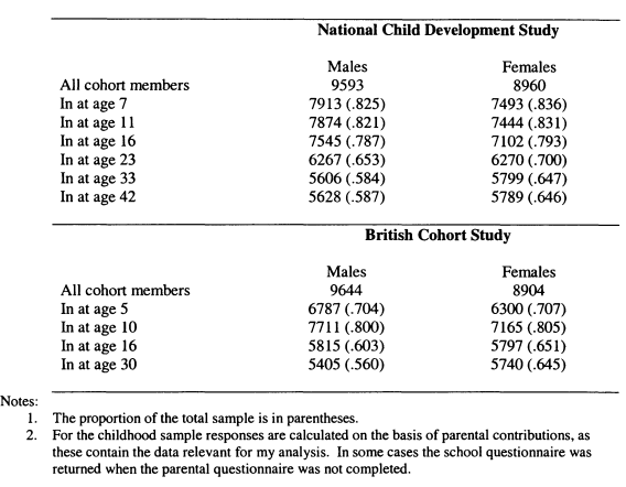

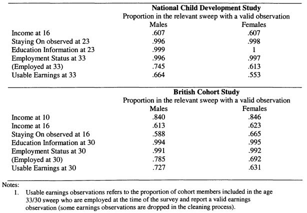

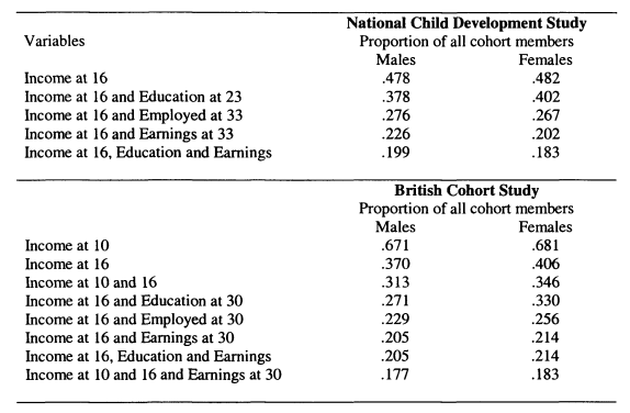

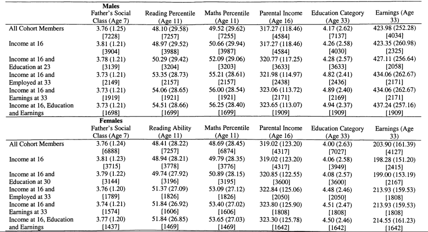

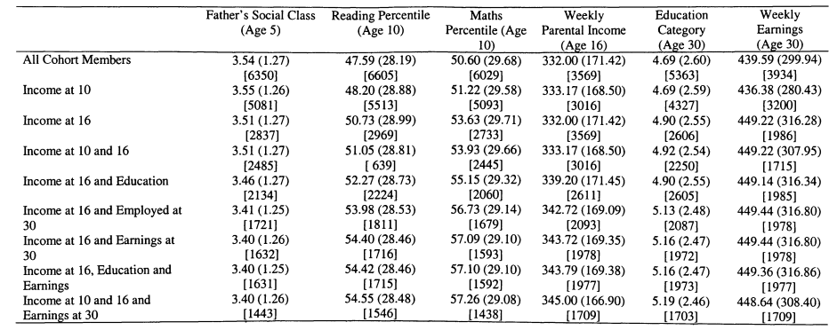

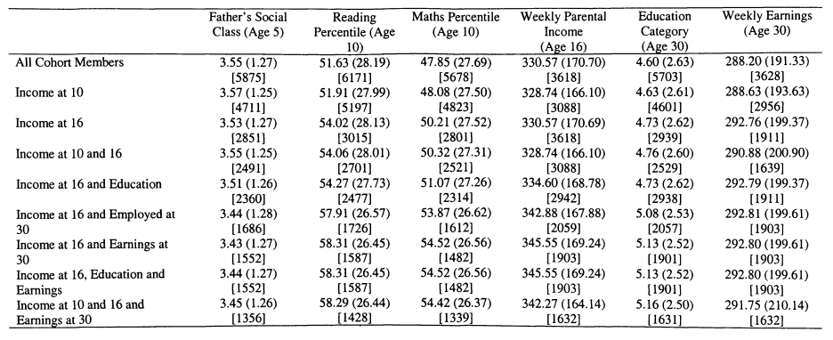
Notes for Tables A4 and A5:
1. Standard deviations are in parentheses.
2. Sample sizes are in square brackets.
3. The father’s social class variable has six categories
1 Professional
2 Intermediate
3 Skilled Non-manual
4 Skilled Manual
5 Semi-skilled
6 Unskilled
A fall in the social class variable therefore indicates an increase in average status.
4. The education variable has nine categories:
0 No qualifications
1 Lower academic e.g. poor CSEs
2 Lower vocational e.g. HGV license
3 Intermediate vocational
4 Intermediate academic e.g. O levels
5 Advanced vocational e.g. GNVQ
6 Advanced academic e.g. A levels
7 Higher vocational e.g. professional qualifications
8 Higher academic e.g. degree
5. Earnings and parental income data is reported in 2000 prices.
References
Alakeson, V. (2005) Too Much, Too Late: Life chances and spending on
education and training Social Market Foundation.
Altonji, J. and T. Dunn (1991) ‘Relationships Amng the Family Incomes and
Labor Market Oucomes of Relatives Research in Labor Economics. Vol.
12, pp. 269-310.
Angrist, J., V. Chemzhukov and I. Femandez-Val (2004) ‘Quantile Regression
Under Misspecification, With An Application to the US Wage Structure’
NBER Working Paper No. 10428.
Annual Abstract of Statistics (2002, 2004), London, The Stationary Office.
Atkinson, A. (1981), ‘On Intergenerational Income Mobility in Britain’, Journal
of Post Keynesian Economics, Vol. 3, pp. 194-218.
Atkinson, A., A. Maynard and C. Trinder (1983), Parents and Children: Incomes
in Two Generations. London: Heinemann.
Becker, G. (1973) ‘A Theory of Marriage: Part 1.’ Journal of Political Economy.
Vol. 81, pp. 813-846.
Becker, G. (1974) ‘A Theory of Marriage: Part 2.’ Journal of Political Economy.
Vol. 82, pp. SI 1-26.
Becker, G and H. G. Lewis. ‘On the interaction between the quantity and quality
of children.’ Journal of Political Economy, Vol. 81, S279-S288.
Becker, G., E. Landes and R. Michael (1979) ‘An Economic Analysis of Marital
Instability’, The Journal of Political Economy. Vol. 85, pp 1141-1188.
Becker, G. and N. Tomes (1986) ‘Human Capital and the Rise and Fall of
Families’ Journal of Labour Economics. Vol. 4, pp. S1-S39.
Becketti, S, W. Gould, L. Lillard and F. Welch. (1988) ‘The PSID after Fourteen
Years: an Evaluation.’ Journal of Labor Economics Vol. 6, pp. 472^192.
Behrman, J and P. Taubman (1985) ‘Intergenerational Earnings Mobility in the
United States: Some Estimates and a Test of Becker’s Intergenerational
Endowments Model’ Review of Economics and Statistics, Vol. 67, pp.
144-151.
Bjorklund, A., B. Bratsburg, T. Eriksson, M. Jantti, R. Naylor, O. Raaum, K.
Roed and E. Osterbacka (2004) ‘Intergenerational earnings mobility in the
Nordic countries, the United Kingdom and the United States’, Draft, Abo
Akademi University, Finland.
Bjorklund, A. and Jantti, M. (1997) ‘Intergenerational Income Mobility in Sweden
Compared to the United States’, American Economic Review Vol. 87, pp.
1009-1018.
Black, S., P. Devereux and K. Salvanes (2005a) ‘The More the Merrier? The
Effect of Family Composition on Children’s Education’, Quarterly Journal
of Economics, Vol. 120, pp. 669-700.
Black, S., P. Devereux and K. Salvanes (2005b) ‘Why the Apple Doesn’t Fall Far:
Understanding Intergenerational Transmission of Human Capital’
American Economic Review, Vol. 95, pp 437-449.
Blackwell, D and D. Lichter (2000) ‘Mate Selection among Married and
Cohabiting Couples’ Journal of Family Issues. Vol. 21, pp. 275-302.
Blanden, J, A. Goodman, P. Gregg and S. Machin (2004) ‘Changes in
Intergenerational Mobility in Britain in M. Corak ed. Generational Income
Mobility in North America and Europe, Cambridge University Press.
Blanden, J and P. Gregg (2004) ‘Family Income and Educational Attainment: A
Review of Approaches and Evidence for Britain’ Oxford Review of
Economic Policy, Vol. 20, pp. 245-264.
Blanden, J. and S. Machin (2004) ‘Educational Inequality and the Expansion of
UK Higher Education’, Scottish Journal of Political Economy. Vol. 51, pp.
230-249.
Blanden, J., P. Gregg and S. Machin (2005) ‘Educational Inequality and
Intergenerational Mobility’ in A. Vignoles and S. Machin (eds) What’s the
Good of Education?, Princeton University Press.
Blundell, R and I. Preston (1998) ‘Consumption Inequality and Income
Uncertainty’ Quarterly Journal of Economics. Vol. 133, pp. 603-640.
Boheim, R. and S. Jenkins (2000) ‘Do Current Income and Annual Income
Measures Provide Different Pictures of Britain’s Income Distribution’
Institute for Social and Economic Research Working Paper, No. 2000-16.
Colchester: University of Essex.
Bratberg, E. & Nilsen, 0 . A. & Vaage, K. (2003) ‘Assessing Changes in
Intergenerational Earnings Mobility,’ IZA Discussion Paper 797.
Brown, C.V. and P. M. Jackson (1990) Public Sector Economics, 3rd Edition,
Oxford.
Brown, C and G. Duncan and F. Stafford (1996) ‘Data Watch: The Panel Study of
Income Dynamics’ Journal of Economic Perspectives. 2, 155-168.
Burdett, K. and M. Coles (1997) ‘Marriage and Class’. The Quarterly Journal of
Economics. Vol. 112, pp. 141-68.
Burdett, K. and M. Coles (1999) ‘Long-term Partnership Formation: Marriage and
Employment.’ The Economic Journal. Vol. 109, pp. F307-F334.
Callender, C. (2003a) ‘Student Financial Support in Higher Education: Access
and Exclusion’ in M. Tight (ed.) Access and Exclusion: International
Perspectives on Higher Education Research, Elsevier Science, London.
Callender, C. (2003b) ‘Attitudes to Debt: School leavers and further education
students’ attitudes to debt and their impact on participation in higher
education’. Report commissioned by Universities UK and the Higher
Education Funding Council.
Cancian, M and D. Reed (1998) ‘Assessing the Effects of Wives’ Earnings on
Family Income Inequality’ Review of Economics and Statistics, 80, 73-79.
Card, D. and T. Lemieux (2000) ‘Drop-out and Enrolment Trends in the Post-War
Period: What Went Wrong in the 1970s?’ NBER Working Paper No.
7658.
Chadwick, L. and G. Solon (2002) ‘Intergenerational Mobility Among
Daughters.’ American Economic Review Vol. 92, pp.335-344.
Chan, T. W. and B. Haplin (2003) ‘Educational Homogamy in Ireland and
Britain’, Sociology Working Paper, 2003-06, University of Oxford.
Chevalier, A (2004) ‘Parental Education and Child’s Education: A Natural
Experiment’ Centre for the Economics of Education Discussion Paper No.
40.
Chevalier A. and C. Harmon, V. O’Sullivan and I. Walker (2005) ‘The Impact of
Parental Income and Education on the Schooling of their Children’
Unpublished, University College Dublin.
Clark-Kauffman, E., G. Duncan and P. Morris (2003) ‘How Welfare Policies
Affect Child and Adolescent Achievement’, American Economic Review.
Vol. 93, pp. 299-303.
Cook, K and A. Demnati (2000) ‘Weighting the Intergenerational Income Data
File’, Social Survey Methods Division, Statistics Canada, Mimeo.
Corak, M. (2004) ‘Do Poor Children Become Poor Adults? Lessons for Public
Policy from a Cross Country Comparison of Generational Earnings
Mobility.’ Mimeo UNICEF Innocenti Research Centre. An expanded
version of the introduction to M. Corak (ed.) Generational Income
Mobility in North America and Europe, Cambridge University Press.
Corak, M. and Heisz, A. (1999) ‘The Intergenerational Income Mobility of
Canadian Men: Evidence from Longitudinal Tax Data.’ Journal of Human
Resources Vol. 34, pp. 504-533.
Corcoran, M. (2001) ‘Mobility, Persistence, and the Consequences of Poverty for
Children: Child and Adult Outcomes.’ In S. Danziger and R. Haveman
(ed.) Understanding Poverty, Russell Sage Foundation and Harvard
University Press.
Couch, K. and T. Dunn (1997) ‘Intergenerational Earnings Mobility in Germany’,
Journal of Human Resources. Vol. 32, pp. 210-232.
Dearden, L., Machin, S. and Reed, H. (1997), ‘Intergenerational Mobility in
Britain’, Economic Journal. Vol. 107, pp. 47-64.
Dearden, L., A. Goodman and P. Saunders (2003) ‘Income and Living Standards’
in E. Ferri, J. Bynner and M. Wadsworth eds. Changing Britain, Changing
Lives.
Denny, K, C. Harmon and V. O’Sullivan (2004) ‘Education, Earnings and Skills:
A Multi-Country Comparison’ Institute for Fiscal Studies Working Paper,
WP04/08.
Dickens, R. (2000) ‘The Evolution of Individual Male Earnings in Britain: 1975-
1995’ Economic Journal. Vol. 107, pp. 47-64.
Dickens, R. and D. Ellwood (2003) ‘Child Poverty in Britain and the United
States’ Economic Journal. Vol. 113, pp. F219-F239.
Dynarski, S. (2004) ‘The New Merit Aid’ Kennedy School of Government
Research Working Paper Series RWP 04-009.
Ermisch, J and M. Francesconi (2000) ‘Cohabitation in Great Britain: not for
long, but here to stay’ Journal of the Roval Statistics Society Series A.
Vol. 163, 153-171.
Ermisch, J. and M. Francesconi (2002) ‘Intergenerational Social Mobility and
Assortative Mating in Britain’, Institute for Social and Economic Research
Working Paper, No. 2002-06. Colchester: University of Essex.
Ermisch and Francesoni (2004) ‘Intergenerational Mobility in Britain: New
Evidence from the British Household Panel Survey’ in M. Corak ed. Generational Income Mobility in North America and Europe, Cambridge
University Press.
Ermisch, J., M. Francesconi and T. Siedler (2004) ‘Intergenerational Social
Mobility and Assortative Mating in Britain’, ISER Mimeo and
forthcoming Economic Journal.
Esping-Andersen, G. (2004) ‘Unequal Opportunities and the Mechanisms of
Social Inheritance’ in in M. Corak (ed.) Generational Income Mobility in
North America and Europe, Cambridge University Press.
Fernandez, R., A. Fogli and C. Olivetti (2004) ‘Mothers and Sons: Preference
Formation and Female Labor Force Dynamics’ Quarterly Journal of
Economics, Vol. 119, pp. 1249-1299.
Fertig, A. (2001). ‘Trends in Intergenerational Earnings Mobility.’ Center for
Research on Child Well-Being Working Paper #01-23, Princeton
University.
Fitzenberger, B and G. Wunderlich (2002) ‘The Changing Life Cycle Pattern in
Female Employment: A Comparison of Germany and the UK’ ZEW
Discussion Paper, Mannheim.
Fitzgerald, J., P. Gottschalk and R. Moffitt (1998a) ‘An Analysis of Sample
Attrition in Panel Data: The Michigan Panel Study of Income Dynamics’
Journal of Human Resources. 33, 251-299.
Fitzgerald, J., P. Gottschalk and R. Moffitt (1998b) ‘An Analysis of the Impact of
Sample Attrition on the Second Generation of Respondents in the Michigan
Panel Study of Income Dynamics’ Journal of Human Resources. 33, 300-
344.
Fortin, N. and S. Lefebvre (1998), ‘Intergenerational Income Mobility in Canada’,
in M. Corak (ed.) Labour Markets, Social Institutions and the Future of
Canada’s Children, Statistics Canada.
Freidman, M. (1957) A Theory of the Consumption Function. Princeton
University Press.
Galindo-Rueda, F and A. Vignoles (forthcoming) ‘The Declining Importance of
Ability in Predicting Educational Attainment’ Journal of Human
Resources.
Galindo-Rueda, F., O. Marcenaro-Gutierrez and A. Vignoles (2004) ‘The
Widening Socio-Economic Gap in UK Higher Education’ National
Institute Economic Review No. 190, pp. 75-88.
Galton, F. (1886), ‘Regression towards mediocrity in hereditary stature’, Journal
of the Anthropological Institute of Great Britain and Ireland. 15, pp. 246-
263.
Gale, D. and L. Shapely (1962) ‘College Admission and the Stability of Marriage’
American Mathematical Monthly. Vol. 69, pp. 9-15.
Gipps, C. and G. Stobart,(1997) Assessment: A Teacher’s Guide to the Issues.
London, Hodder and Stoughton.
Glenn, N., A. Ross and J. Tully (1974) ‘Patterns of Intergenerational Mobility of
Daughters Through Marriage.’ American Sociological Review. Vol. 39,
pp.683-699.
Goldberger, A. (1989) ‘Economic and Mechanical Models of Intergenerational
Transmission’ American Economic Review, 79, 504-513.
Goering, J. and J. Feins Eds. (2003) Choosing a Better Life? Evaluating the
Moving to Opportunity Social Experiment, Urban Institute Press,
Washington DC.
Goldthorpe, J and C. Mills (2004) ‘Trends in Intergenerational Class Mobility in
Britain in the late Twentieth Century’ in R. Breen (ed.) Social Mobility in
Europe, Oxford University Press.
Goode, W. J. (1982) The Family Second Ed. Englewood Cliffs, NJ: Prentice Hall.
Goodman, A and G. Kaplan (2003) “ Study Now, pay later’ or ‘HE for Free’? An
Assessment of alternative proposals for higher education finance’ Institute
for Fiscal Studies Commentary No. 94.
Gottschalk, P. and T. Smeeding (1997) ‘Cross-National Comparisons of Earnings
and Income Inequality’ Journal of Economic Literature. Vol. 35, pp. 633-
687.
Grawe, N. (2003) ‘Lifecycle Bias in the Estimation of Intergenerational Income
Mobility.’ Statistics Canada Analytical Studies Branch Working Paper
Series, no 207.
Grawe, N. (2004a) ‘Reconsidering the Use of Non linearities in Intergenerational
Earnings Mobility as a Test for Credit Constraints’ Journal of Human
Resources. Vol. 34, pp. 813-827.
Grawe, N. (2004b) ‘Intergenerational Mobility for Whom? The Experience of
High and Low Earning Sons in International Perspective’ in M. Corak
(ed.) Generational Income Mobility in North America and Europe,
Cambridge University Press.
Grawe, N. (2004c) ‘The 3-day Week of 1974 and Earnings Data Reliability in the
Family Expenditure Survey and the National Child Development Survey’
Oxford Bulletin of Economics and Statistics. Vol. 66, pp. 567-579.
Grawe, N. and C. Mulligan (2002), ‘Economic Interpretations of Intergenerational
Correlations’. Journal of Economic Perspectives, Vol. 16, pp.45-58.
Greenaway, D. and M. Haynes (2003) ‘Funding Higher Education in the UK: The
Role of Fees and Loans’, Economic Journal. 113, F150-F167.
Gregg, P. and S. Machin (1999) ‘Childhood Disadvantage and Success or Failure
in the Labour Market’, in D. Blanchflower and R. Freeman (eds.) Youth
Employment and Joblessness in Advanced Countries, National Bureau of
Economic Research, Cambridge, MA.
Gregg, P., S. Machin and A. Manning (2004) ‘Mobility and Joblessness’ in D.
Card, R. Blundell and R. Freeman (eds.) Seeking a Premier Economy: The
Economic Effects of British Economic Reforms 1980-2000, National
Bureau of Economic Research, Cambridge, MA.
Gregg, P., J. Waldfogel and E. Washbrook (2005) ‘That’s The Way Goes:
Expenditure Patterns as Real Incomes Rise for the Poorest Families with
Chidlren’ in J. Hills and K. Stewart A More Equal Society? New Labour,
Poverty, Inequality and Exclusion, Policy Press.
Haider, S and G. Solon (2004) ‘Life-Cycle Variation in the Association between
Current and Lifetime Earnings.’ Unpublished, University of Michigan.
Haisken-DeNew, J. and J. Frick (2000) ‘Desk-Top Companion to the German
Socio-Economic Panel Study: Version 6.0’, DIW Berlin.
Harkness, S., S. Machin and J. Waldfogel (1997) ‘Evaluating the pin money
hypothesis: The relationship between women’s labour market activity,
family income and poverty in Britain, Journal of Population Economics.
Vol. 10, pp. 137-158.
Heckman, J. (1979) ‘Sample Selection Bias as a Specification Error’
Econometrica, Vol. 47, 1, pp. 153-162.
HEFCE (2005) Young Participation in Higher Education.
Hout, M. (2003) ‘The Inequality-Mobility Paradox: The Lack of Correlation
Between Social Mobility and Equality’ New Economy. Vol. 10, pp. 205-
207.
Hout, M. (2004) ‘How Inequality may Affect Intergenerational Mobility’ in ed. K.
Neckerman (ed.) Social Inequality, Russell Sage Foundation, New York.
Jepsen, L and C. Jepsen (2002) ‘An Empirical Analysis of the Matching Patterns
of Same-Sex and Opposite-Sex Couples’ Demography, Vol. 39, pp. 435-
453.
Kalmijn, M. (1998) ‘Intermarriage and Homogamy: Causes, Patterns, Trends’
Annual Review of Sociology. Vol. 24, pp. 395-541.
Kane, T. (1999) The Price of Admission: Rethinking How Americans Pay for
College, Brookings Press, Washington.
Katz, L. and D. Autor (1999) ‘Inequality in the Labour Market’ in O. Ashenfelter
and D. Card eds Handbook of Labour Economics, North Holland.
Korenman, S. and D. Sanders (1991) ‘Does marriage really make men more
productive?’ Journal of Human Resources, Vol. 26, pp. 282-307.
Jackman, R. and S. Savour (1999) “ Has Britain solved the ‘regional problem’?”
In P.Gregg and J. Wadsworth (eds) The State of Working Britain,
Manchester University Press.
Lam, D (1988) ‘Marriage Markets and Assortative Mating with Household Public
Goods: Theoretical Results and Empirical Implications’, The Journal of
Human Resources, Vol. 23, pp. 462-487.
Lam, D. and R. Schoeni (1993) ‘Effects of Family Background on Earnings and
Returns to Schooling’ Journal of Political Economy, Vol. 101, pp. 710-
740.
Lam, D. and R. Schoeni (1994) ‘Family Ties and Labor Markets in the United
States and Brazil’ Journal of Human Resources, Vol. 29, pp. 1235-1258.
Lee, C.-I. and G. Solon (2004) ‘Trends in Intergenerational Income Mobility’
Unpublished, University of Michigan.
Levine, D. and B. Mazumder (2002) ‘Choosing the Right Parents: Changes in the
Intergenerational Transmission of Inequality – Between 1980 and the
Early 1990s’, Working Paper 2002-08, Federal Reserve Bank of Chicago.
Levy, D. and Duncan, G. (2001) Using Siblings to Assess the Effect of Childhood
Family Income on Completed Schooling, Joint Centre for Poverty
Research Working Paper, North Western University.
Lillard, D. P. Giles, M. Grabka, and M. Schroeder (2002) ‘Codebook for the
Cross-National Equivalent File 1980-2001, BHPS – GSOEP – PSID –
SLID’, Cornell University. Available at
http://www.human.comell.edu/pam/gsoep/equivfil.cfm.
Machin, S. (1999) ‘Wage Inequality in the 1970s, 1980s and 1990s.’ In P.Gregg
and J. Wadsworth (eds) The State of Working Britain, Manchester
University Press.
Magee, L. J. Burbidge and L. Robb (2000) ‘The Correlation between Husband’s
and Wive’s Education: Canada, 1971-1996’, QSEP Research Report no.
353, McMaster University.
Manski, C. (1992) ‘Income and Higher Education’ Focus, University of
Wisconsin-Madison, Institute for Research on Poverty, 13, 3, pp. 14-19.
Manski, C. (Forthcoming) ‘Partial identification with missing data: concepts and
findings’ International Journal of Approximate Reasoning.
Mare, R (1991) ‘Five Decades of Educational Assortative Mating’ American
Sociological Review. 56, ppl5-32.
Mayer, S. (1997) What Money Can’t Buy: Family Income and Children’s Life
Chances, Harvard University Press.
Mayer, S and L. Lopoo (2004) ‘What Do Trends in Intergenerational Economic
Mobility of Sons and Daughters in the United States Mean?’ in M. Corak
ed. Generational Income mobility in North America and Europe,
Cambridge University Press.
Mayer, S and L. Lopoo (forthcoming) ‘Has the Intergenerational Transmission of
Economic Status Changed’, Journal of Human Resources.
Mazumder, B. (2001). ‘Earnings Mobility in the US: a New Look at
Intergenerational Mobility.’ Federal Reserve Bank of Chicago Working
Paper 2001-18.
McClements, L. (1977) ‘Equivalence Scales for Children’ Journal of Public
Economics. 8, 191-210.
McNally, S (forthcoming) ‘Reforms to Schooling in the UK: A Review of Some
Major Reforms and their Evaluation’ German Economic Review, Special
Issue on Education.
Mickelwright, J. (1986) ‘A Note on Household Income Data in NCDS 3’ National
Child Development Study User Support Group’, City University.
Mincer, J. (1958) ‘Investment in Human Capital and the Personal Income
Distribution’ Journal of Political Economy, Vol. 66, pp. 281-302.
Mincer, J. (1974) Schooling, Experience and Earnings New York: National
Bureau of Economic Research.
Minicozzi, A (2002) ‘Estimating Intergenerational Earnings Mobility for
Daughters’ University of Texas at Austin, Mimeo.
Mortensen, D. (1988) ‘Matching: Finding a Partner for Life or Otherwise’ The
American Journal of Sociology. Vol. 94, pp. S215-S240.
Mulligan, C. (1997) Parental Priorities and Economic Inequality University of
Chicago Press.
Mulligan, C. (1999) ‘Galton versus the Human Capital Approach to Inheritance.’
Journal of Political Economy. Vol. 107, pp. S184-S224.
Mulligan, C. and Y. Rubinstein (2004) ‘The Closing of the Gender Gap as a Roy
Model Illusion’, NBER Working Paper No. 10892.
Mulligan, C. and Y. Rubinstein (2005) ‘Selection, Investment, and Women’s
Relative Wages Since 1975’, NBER Working Paper No. 11159.
Oreopoulos, P., M. Page and A. Stevens (2003) ‘Does Human Capital Transfer
from Parent to Child? The Intergenerational Effects of Compulsory
Schooling’, University of Toronto, Mimeo.
Oreopoulos, P. (2003) ‘The Long-Run Consequences of Growing-Up in a Poor
Neighborhood’ Ouaterlv Journal of Economics. Vol. 118, pp. 1533-1575.
Osterbacka, E. (2004) ‘Mechanisms behind Intergenerational Earnings
Correlation in Finland 1985-1955’ Paper presented at the 2004 Conference
of the International Association for Research in Income and Wealth, Cork.
Osterbacka, E. (2001) ‘Family Background and Economic Status in Finland
Scandinavian Journal of Economics Vol. 103, pp. 467-484.
Pencavel, J. (1998) ‘Assortative Mating by Schooling and the Work Behaviour of
Wives and Husbands’ American Economic Review, Papers and
Proceedings, Vol. 88, pp. 326-329.
Perisco, N., A. Postlewaite and D. Silverman (2004) ‘The Effect of Adolescent
Experience on Labour Market Outcomes: The Case of Height’ Journal of
Political Economy. Vol. 112, pp. 1019-1053.
Pischke, J-S. (1993) ‘Assimilation and the Earnings of Guestworkers in Germany’
MIT, Mimeo.
Plewis, I., L. Calderwood, D. Hawkes and G. Nathan (2004) ‘Changes in the
NCDS and BCS70 Populations and Samples Over Time’ National Child
Development and 1970 British Cohort Study Technical Report, Centre for
Longitudinal Studies.
Reville, R. (1995) ‘Intertemporal and Life Cycle Variation in Measured
Intergenerational Mobility’ Unpublished, RAND.
R0ed, K. and O. Raaum (2003) ‘Administrative Registers – Unexplored
Reservoirs of Scientific Knowledge?’, Economic Journal. Vol. 113, pp.
F258-F281
Sewell, W and R. Hauser (1975) Education, Occupation and Earnings:
Achievement in the Early Career, New York: Academic Press.
Shea, J. (2000) ‘Does Parent’s Money Matter?’ Journal of Public Economics. Vol.
77, pp. 155-184.
Shimer, R and L. Smith (2000) ‘Assortative Matching and Search’ Econometrica,
Vol. 68, pp. 343-369.
Singh, S. and G. Maddala (1976) ‘A Function for Size Distribution of Incomes’
Econometrica. Vol. 44, pp. 963-970.
Solon, G. (1989), ‘Biases in the Estimation of Intergenerational Earnings
Correlations’, Review of Economics and Statistics, Vol. 71, pp. 172-174.
Solon, G. (1992) ‘Intergenerational Income Mobility in the United States.’
American Economic Review Vol. 82, pp. 383-408.
Solon, G. (1999), ‘Intergenerational Mobility in the Labor Market’, in O.
Ashenfelter and D. Card (eds.), Handbook of Labor Economics, Volume
3A, North Holland.
Solon, G. (2002) ‘Cross-Country Differences in Intergenerational Earnings
Mobility’, Journal of Economic Perspectives. Vol. 16, pp. 59-66.
Solon, G. (2004) ‘A Model of Intergenerational Mobility Variation over Time and
Place,’ in M. Corak ed. Generational Income mobility in North America
and Europe, Cambridge University Press.
Speiss, M and M. Pannenberg (2003) ‘Documentation of Sample Sizes and Panel
Attrition in the German Socio Economic Panel (1984 until 2002)’, Research
Note 28, DIW Berlin.
Steedman, H., McIntosh, S. and Green, A. (2004) ‘International Comparisons of
Qualifications: Skills Audit Update,’ DfES Research Report 548.
Statistics Canada (1999) ‘Earnings of Men and Women, 1997’, Income Statistics
Division, Statistics Canada, Ottawa.
Vella, F. (1998) ‘Estimating Models with Sample Selection Bias: A Survey’ The
Journal of Human Resources. Vol. 33 pp.127-169.
Weiss, Y and R. Willis (1997) ‘Match Quality, New Information, and Marital
Dissolution’ Journal of Labor Economics. Vol. 15, pp. S293-S329.
Wiegand, J. (1999) ‘Intergenerational Earnings Mobility in Germany’ University
College London, Mimeo.
Willen, P., I. Hendel and J. Shapiro (2004) ‘Educational Opportunity and Income
Inequality’ NBER Working Paper 10879.
Wu, Z. (2000) Cohabitation: An Alternative Form of Family Living, Oxford
University Press, Ontario.
Zimmerman, D. (1992) ‘Regression Toward Mediocrity in Economic Stature’,
American Economic Review, Vol. 82, pp. 409-429.